©2011 O’Reilly Media, Inc. O’Reilly logo is a registered trademark of O’Reilly Media, Inc.
Learn how to turn
data into decisions.
From startups to the Fortune 500,
smart companies are betting on
data-driven insight, seizing the
opportunities that are emerging
from the convergence of four
powerful trends:
n New methods of collecting, managing, and analyzing data
n Cloud computing that offers inexpensive storage and flexible,
on-demand computing power for massive data sets
n Visualization techniques that turn complex data into images
that tell a compelling story
n Tools that make the power of data available to anyone
Get control over big data and turn it into insight with O’Reilly’s Strata offerings. Find the inspiration and information to create new products or revive existing ones, understand customer behavior, and get the data edge.
Andrew Collette
Python and HDF5
by Andrew Collette
Copyright © 2014 Andrew Collette. All rights reserved. Printed in the United States of America.
Published by O’Reilly Media, Inc., 1005 Gravenstein Highway North, Sebastopol, CA 95472.
O’Reilly books may be purchased for educational, business, or sales promotional use. Online editions are also available for most titles (http://my.safaribooksonline.com). For more information, contact our corporate/ institutional sales department: 800-998-9938 or [email protected].
Editors: Meghan Blanchette and Rachel Roumeliotis
Production Editor: Nicole Shelby
Copyeditor: Charles Roumeliotis
Proofreader: Rachel Leach
Indexer: WordCo Indexing Services
Cover Designer: Karen Montgomery
Interior Designer: David Futato
Illustrator: Kara Ebrahim November 2013: First Edition
Revision History for the First Edition:
2013-10-18: First release
See http://oreilly.com/catalog/errata.csp?isbn=9781449367831 for release details.
Nutshell Handbook, the Nutshell Handbook logo, and the O’Reilly logo are registered trademarks of O’Reilly Media, Inc. Python and HDF5, the images of Parrot Crossbills, and related trade dress are trademarks of O’Reilly Media, Inc.
Many of the designations used by manufacturers and sellers to distinguish their products are claimed as trademarks. Where those designations appear in this book, and O’Reilly Media, Inc., was aware of a trade‐ mark claim, the designations have been printed in caps or initial caps.
While every precaution has been taken in the preparation of this book, the publisher and author assume no responsibility for errors or omissions, or for damages resulting from the use of the information contained herein.
Table of Contents
Preface. . . xi
1. Introduction. . . 1
Python and HDF5 2
Organizing Data and Metadata 2
Coping with Large Data Volumes 3
What Exactly Is HDF5? 4
HDF5: The File 5
HDF5: The Library 6
HDF5: The Ecosystem 6
2. Getting Started. . . 7
HDF5 Basics 7
Setting Up 8
Python 2 or Python 3? 8
Code Examples 9
NumPy 10
HDF5 and h5py 11
IPython 11
Timing and Optimization 12
The HDF5 Tools 14
HDFView 14
ViTables 15
Command Line Tools 15
Your First HDF5 File 17
Use as a Context Manager 18
File Drivers 18
The User Block 19
3. Working with Datasets. . . 21
Dataset Basics 21
Type and Shape 21
Reading and Writing 22
Creating Empty Datasets 23
Saving Space with Explicit Storage Types 23
Automatic Type Conversion and Direct Reads 24
Reading with astype 25
Reshaping an Existing Array 26
Fill Values 26
Reading and Writing Data 27
Using Slicing Effectively 27
Start-Stop-Step Indexing 29
Multidimensional and Scalar Slicing 30
Boolean Indexing 31
Coordinate Lists 32
Automatic Broadcasting 33
Reading Directly into an Existing Array 34
A Note on Data Types 35
Resizing Datasets 36
Creating Resizable Datasets 37
Data Shuffling with resize 38
When and How to Use resize 39
4. How Chunking and Compression Can Help You. . . 41
Contiguous Storage 41
Chunked Storage 43
Setting the Chunk Shape 45
Auto-Chunking 45
Manually Picking a Shape 45
Performance Example: Resizable Datasets 46
Filters and Compression 48
The Filter Pipeline 48
Compression Filters 49
GZIP/DEFLATE Compression 50
SZIP Compression 50
LZF Compression 51
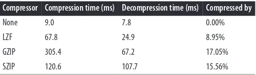
Performance 51
Other Filters 52
FLETCHER32 Filter 53
Third-Party Filters 54
5. Groups, Links, and Iteration: The “H” in HDF5. . . 55
The Root Group and Subgroups 55
Group Basics 56
Dictionary-Style Access 56
Special Properties 57
Working with Links 57
Hard Links 57
Free Space and Repacking 59
Soft Links 59
External Links 61
A Note on Object Names 62
Using get to Determine Object Types 63
Using require to Simplify Your Application 64
Iteration and Containership 65
How Groups Are Actually Stored 65
Dictionary-Style Iteration 66
Containership Testing 67
Multilevel Iteration with the Visitor Pattern 68
Visit by Name 68
Multiple Links and visit 69
Visiting Items 70
Canceling Iteration: A Simple Search Mechanism 70
Copying Objects 71
Single-File Copying 71
Object Comparison and Hashing 72
6. Storing Metadata with Attributes. . . 75
Attribute Basics 75
Type Guessing 77
Strings and File Compatibility 78
Python Objects 80
Explicit Typing 80
Real-World Example: Accelerator Particle Database 82
Application Format on Top of HDF5 82
Analyzing the Data 84
7. More About Types. . . 87
The HDF5 Type System 87
Integers and Floats 88
Fixed-Length Strings 89
Variable-Length Strings 89
The vlen String Data Type 90
Working with vlen String Datasets 91
Byte Versus Unicode Strings 91
Using Unicode Strings 92
Don’t Store Binary Data in Strings! 93
Future-Proofing Your Python 2 Application 93
Compound Types 93
Complex Numbers 95
Enumerated Types 95
Booleans 96
The array Type 97
Opaque Types 98
Dates and Times 99
8. Organizing Data with References, Types, and Dimension Scales. . . 101
Object References 101
Creating and Resolving References 101
References as “Unbreakable” Links 102
References as Data 103
Region References 104
Creating Region References and Reading 104
Fancy Indexing 105
Finding Datasets with Region References 106
Named Types 106
The Datatype Object 107
Linking to Named Types 107
Managing Named Types 108
Dimension Scales 108
Creating Dimension Scales 109
Attaching Scales to a Dataset 110
9. Concurrency: Parallel HDF5, Threading, and Multiprocessing. . . 113
Python Parallel Basics 113
Threading 114
Multiprocessing 116
MPI and Parallel HDF5 119
A Very Quick Introduction to MPI 120
MPI-Based HDF5 Program 121
Atomicity Gotchas 123
10. Next Steps. . . 127
Asking for Help 127
Contributing 127
Index. . . 129
Preface
Over the past several years, Python has emerged as a credible alternative to scientific analysis environments like IDL or MATLAB. Stable core packages now exist for han‐ dling numerical arrays (NumPy), analysis (SciPy), and plotting (matplotlib). A huge selection of more specialized software is also available, reducing the amount of work necessary to write scientific code while also increasing the quality of results.
As Python is increasingly used to handle large numerical datasets, more emphasis has been placed on the use of standard formats for data storage and communication. HDF5, the most recent version of the “Hierarchical Data Format” originally developed at the National Center for Supercomputing Applications (NCSA), has rapidly emerged as the mechanism of choice for storing scientific data in Python. At the same time, many researchers who use (or are interested in using) HDF5 have been drawn to Python for its ease of use and rapid development capabilities.
This book provides an introduction to using HDF5 from Python, and is designed to be useful to anyone with a basic background in Python data analysis. Only familiarity with Python and NumPy is assumed. Special emphasis is placed on the native HDF5 feature set, rather than higher-level abstractions on the Python side, to make the book as useful as possible for creating portable files.
Finally, this book is intended to support both users of Python 2 and Python 3. While the examples are written for Python 2, any differences that may trip you up are noted in the text.
Conventions Used in This Book
The following typographical conventions are used in this book:
Italic
Indicates new terms, URLs, email addresses, filenames, and file extensions.
Constant width
Used for program listings, as well as within paragraphs to refer to program elements such as variable or function names, databases, data types, environment variables, statements, and keywords.
Constant width bold
Shows commands or other text that should be typed literally by the user.
Constant width italic
Shows text that should be replaced with user-supplied values or by values deter‐ mined by context.
This icon signifies a tip, suggestion, or general note.
This icon indicates a warning or caution.
Using Code Examples
This book is here to help you get your job done. In general, if example code is offered with this book, you may use it in your programs and documentation. You do not need to contact us for permission unless you’re reproducing a significant portion of the code. For example, writing a program that uses several chunks of code from this book does not require permission. Selling or distributing a CD-ROM of examples from O’Reilly books does require permission. Answering a question by citing this book and quoting example code does not require permission. Incorporating a significant amount of ex‐ ample code from this book into your product’s documentation does require permission.
We appreciate, but do not require, attribution. An attribution usually includes the title, author, publisher, and ISBN. For example: “Python and HDF5 by Andrew Collette (O’Reilly). Copyright 2014 Andrew Collette, 978-1-449-36783-1.”
If you feel your use of code examples falls outside fair use or the permission given above, feel free to contact us at [email protected].
Safari® Books Online
Technology professionals, software developers, web designers, and business and crea‐ tive professionals use Safari Books Online as their primary resource for research, prob‐ lem solving, learning, and certification training.
Safari Books Online offers a range of product mixes and pricing programs for organi‐ zations, government agencies, and individuals. Subscribers have access to thousands of books, training videos, and prepublication manuscripts in one fully searchable database from publishers like O’Reilly Media, Prentice Hall Professional, Addison-Wesley Pro‐ fessional, Microsoft Press, Sams, Que, Peachpit Press, Focal Press, Cisco Press, John Wiley & Sons, Syngress, Morgan Kaufmann, IBM Redbooks, Packt, Adobe Press, FT Press, Apress, Manning, New Riders, McGraw-Hill, Jones & Bartlett, Course Technol‐ ogy, and dozens more. For more information about Safari Books Online, please visit us online.
How to Contact Us
Please address comments and questions concerning this book to the publisher:
O’Reilly Media, Inc.
1005 Gravenstein Highway North Sebastopol, CA 95472
800-998-9938 (in the United States or Canada) 707-829-0515 (international or local)
707-829-0104 (fax)
We have a web page for this book, where we list errata, examples, and any additional information. You can access this page at http://oreil.ly/python-HDF5.
To comment or ask technical questions about this book, send email to bookques [email protected].
For more information about our books, courses, conferences, and news, see our website at http://www.oreilly.com.
Find us on Facebook: http://facebook.com/oreilly
Follow us on Twitter: http://twitter.com/oreillymedia
Watch us on YouTube: http://www.youtube.com/oreillymedia
Acknowledgments
I would like to thank Quincey Koziol, Elena Pourmal, Gerd Heber, and the others at the HDF Group for supporting the use of HDF5 by the Python community. This book benefited greatly from reviewer comments, including those by Eli Bressert and Anthony Scopatz, as well as the dedication and guidance of O’Reilly editor Meghan Blanchette.
CHAPTER 1
Introduction
When I was a graduate student, I had a serious problem: a brand-new dataset, made up of millions of data points collected painstakingly over a full week on a nationally rec‐ ognized plasma research device, that contained values that were much too small.
About 40 orders of magnitude too small.
My advisor and I huddled in his office, in front of the shiny new G5 Power Mac that ran our visualization suite, and tried to figure out what was wrong. The data had been acquired correctly from the machine. It looked like the original raw file from the ex‐ periment’s digitizer was fine. I had written a (very large) script in the IDL programming language on my Thinkpad laptop to turn the raw data into files the visualization tool could use. This in-house format was simplicity itself: just a short fixed-width header and then a binary dump of the floating-point data. Even so, I spent another hour or so writing a program to verify and plot the files on my laptop. They were fine. And yet, when loaded into the visualizer, all the data that looked so beautiful in IDL turned into a featureless, unstructured mush of values all around 10-41.
Finally it came to us: both the digitizer machines and my Thinkpad used the “little-endian” format to represent floating-point numbers, in contrast to the “big-“little-endian” format of the G5 Mac. Raw values written on one machine couldn’t be read on the other, and vice versa. I remember thinking that’s so stupid (among other less polite variations). Learning that this problem was so common that IDL supplied a special routine to deal with it (SWAP_ENDIAN) did not improve my mood.
At the time, I didn’t care that much about the details of how my data was stored. This incident and others like it changed my mind. As a scientist, I eventually came to rec‐ ognize that the choices we make for organizing and storing our data are also choices about communication. Not only do standard, well-designed formats make life easier for individuals (and eliminate silly time-wasters like the “endian” problem), but they make it possible to share data with a global audience.
Python and HDF5
In the Python world, consensus is rapidly converging on Hierarchical Data Format version 5, or “HDF5,” as the standard mechanism for storing large quantities of nu‐ merical data. As data volumes get larger, organization of data becomes increasingly important; features in HDF5 like named datasets (Chapter 3), hierarchically organized groups (Chapter 5), and user-defined metadata “attributes” (Chapter 6) become essen‐ tial to the analysis process.
Structured, “self-describing” formats like HDF5 are a natural complement to Python. Two production-ready, feature-rich interface packages exist for HDF5, h5py, and PyT‐ ables, along with a number of smaller special-purpose wrappers.
Organizing Data and Metadata
Here’s a simple example of how HDF5’s structuring capability can help an application. Don’t worry too much about the details; later chapters explain both the details of how the file is structured, and how to use the HDF5 API from Python. Consider this a taste of what HDF5 can do for your application. If you want to follow along, you’ll need Python 2 with NumPy installed (see Chapter 2).
Suppose we have a NumPy array that represents some data from an experiment:
>>> import numpy as np
>>> temperature = np.random.random(1024) >>> temperature
array([ 0.44149738, 0.7407523 , 0.44243584, ..., 0.19018119, 0.64844851, 0.55660748])
Let’s also imagine that these data points were recorded from a weather station that sampled the temperature, say, every 10 seconds. In order to make sense of the data, we have to record that sampling interval, or “delta-T,” somewhere. For now we’ll put it in a Python variable:
>>> dt = 10.0
The data acquisition started at a particular time, which we will also need to record. And of course, we have to know that the data came from Weather Station 15:
>>> start_time = 1375204299 # in Unix time
>>> station = 15
We could use the built-in NumPy function np.savez to store these values on disk. This simple function saves the values as NumPy arrays, packed together in a ZIP file with associated names:
>>> np.savez("weather.npz", data=temperature, start_time=start_time, station=
station)
>>> out = np.load("weather.npz") >>> out["data"]
array([ 0.44149738, 0.7407523 , 0.44243584, ..., 0.19018119, 0.64844851, 0.55660748])
>>> out["start_time"] array(1375204299) >>> out["station"] array(15)
So far so good. But what if we have more than one quantity per station? Say there’s also wind speed data to record?
>>> wind = np.random.random(2048)
>>> dt_wind = 5.0 # Wind sampled every 5 seconds
And suppose we have multiple stations. We could introduce some kind of naming con‐ vention, I suppose: “wind_15” for the wind values from station 15, and things like “dt_wind_15” for the sampling interval. Or we could use multiple files…
In contrast, here’s how this application might approach storage with HDF5:
>>> import h5py
>>> f = h5py.File("weather.hdf5") >>> f["/15/temperature"] = temperature
>>> f["/15/temperature"].attrs["dt"] = 10.0
>>> f["/15/temperature"].attrs["start_time"] = 1375204299 >>> f["/15/wind"] = wind
>>> f["/15/wind"].attrs["dt"] = 5.0
--->>> f["/20/temperature"] = temperature_from_station_20
---(and so on)
This example illustrates two of the “killer features” of HDF5: organization in hierarchical groups and attributes. Groups, like folders in a filesystem, let you store related datasets together. In this case, temperature and wind measurements from the same weather station are stored together under groups named “/15,” “/20,” etc. Attributes let you attach descriptive metadata directly to the data it describes. So if you give this file to a colleague, she can easily discover the information needed to make sense of the data:
>>> dataset = f["/15/temperature"]
>>> for key, value in dataset.attrs.iteritems(): ... print "%s: %s" % (key, value)
dt: 10.0
start_time: 1375204299
Coping with Large Data Volumes
As a high-level “glue” language, Python is increasingly being used for rapid visualization of big datasets and to coordinate large-scale computations that run in compiled lan‐
guages like C and FORTRAN. It’s now relatively common to deal with datasets hundreds of gigabytes or even terabytes in size; HDF5 itself can scale up to exabytes.
On all but the biggest machines, it’s not feasible to load such datasets directly into memory. One of HDF5’s greatest strengths is its support for subsetting and partial I/O. For example, let’s take the 1024-element “temperature” dataset we created earlier:
>>> dataset = f["/15/temperature"]
Here, the object named dataset is a proxy object representing an HDF5 dataset. It supports array-like slicing operations, which will be familiar to frequent NumPy users:
>>> dataset[0:10]
array([ 0.44149738, 0.7407523 , 0.44243584, 0.3100173 , 0.04552416, 0.43933469, 0.28550775, 0.76152561, 0.79451732, 0.32603454]) >>> dataset[0:10:2]
array([ 0.44149738, 0.44243584, 0.04552416, 0.28550775, 0.79451732])
Keep in mind that the actual data lives on disk; when slicing is applied to an HDF5 dataset, the appropriate data is found and loaded into memory. Slicing in this fashion leverages the underlying subsetting capabilities of HDF5 and is consequently very fast.
Another great thing about HDF5 is that you have control over how storage is allocated. For example, except for some metadata, a brand new dataset takes zero space, and by default bytes are only used on disk to hold the data you actually write.
For example, here’s a 2-terabyte dataset you can create on just about any computer:
>>> big_dataset = f.create_dataset("big", shape=(1024, 1024, 1024, 512),
dtype='float32')
Although no storage is yet allocated, the entire “space” of the dataset is available to us. We can write anywhere in the dataset, and only the bytes on disk necessary to hold the data are used:
>>> big_dataset[344, 678, 23, 36] = 42.0
When storage is at a premium, you can even use transparent compression on a dataset-by-dataset basis (see Chapter 4):
>>> compressed_dataset = f.create_dataset("comp", shape=(1024,), dtype='int32',
compression='gzip')
>>> compressed_dataset[:] = np.arange(1024) >>> compressed_dataset[:]
array([ 0, 1, 2, ..., 1021, 1022, 1023])
What Exactly Is HDF5?
It’s quite different from SQL-style relational databases. HDF5 has quite a few organi‐ zational tricks up its sleeve (see Chapter 8, for example), but if you find yourself needing to enforce relationships between values in various tables, or wanting to perform JOINs on your data, a relational database is probably more appropriate. Likewise, for tiny 1D datasets you need to be able to read on machines without HDF5 installed. Text formats like CSV (with all their warts) are a reasonable alternative.
HDF5 is just about perfect if you make minimal use of relational features and have a need for very high performance, partial I/O, hierarchical organization, and arbitrary metadata.
So what, specifically, is “HDF5”? I would argue it consists of three things:
1. A file specification and associated data model.
2. A standard library with API access available from C, C++, Java, Python, and others.
3. A software ecosystem, consisting of both client programs using HDF5 and “analysis platforms” like MATLAB, IDL, and Python.
HDF5: The File
In the preceding brief examples, you saw the three main elements of the HDF5 data model: datasets, array-like objects that store your numerical data on disk; groups, hier‐ archical containers that store datasets and other groups; and attributes, user-defined bits of metadata that can be attached to datasets (and groups!).
Using these basic abstractions, users can build specific “application formats” that orga‐ nize data in a method appropriate for the problem domain. For example, our “weather station” code used one group for each station, and separate datasets for each measured parameter, with attributes to hold additional information about what the datasets mean. It’s very common for laboratories or other organizations to agree on such a “format-within-a-format” that specifies what arrangement of groups, datasets, and attributes are to be used to store information.
Since HDF5 takes care of all cross-platform issues like endianness, sharing data with other groups becomes a simple matter of manipulating groups, datasets, and attributes to get the desired result. And because the files are self-describing, even knowing about the application format isn’t usually necessary to get data out of the file. You can simply open the file and explore its contents:
>>> f.keys()
[u'15', u'big', u'comp'] >>> f["/15"].keys() [u'temperature', u'wind']
Anyone who has spent hours fiddling with byte-offsets while trying to read “simple” binary formats can appreciate this.
Finally, the low-level byte layout of an HDF5 file on disk is an open specification. There are no mysteries about how it works, in contrast to proprietary binary formats. And although people typically use the library provided by the HDF Group to access files, nothing prevents you from writing your own reader if you want.
HDF5: The Library
The HDF5 file specification and open source library is maintained by the HDF Group, a nonprofit organization headquartered in Champaign, Illinois. Formerly part of the University of Illinois Urbana-Champaign, the HDF Group’s primary product is the HDF5 software library.
Written in C, with additional bindings for C++ and Java, this library is what people usually mean when they say “HDF5.” Both of the most popular Python interfaces, PyTables and h5py, are designed to use the C library provided by the HDF Group.
One important point to make is that this library is actively maintained, and the devel‐ opers place a strong emphasis on backwards compatibility. This applies to both the files the library produces and also to programs that use the API. File compatibility is a must for an archival format like HDF5. Such careful attention to API compatibility is the main reason that packages like h5py and PyTables have been able to get traction with many different versions of HDF5 installed in the wild.
You should have confidence when using HDF5 for scientific data storage, including long-term storage. And since both the library and format are open source, your files will be readable even if a meteor takes out Illinois.
HDF5: The Ecosystem
Finally, one aspect that makes HDF5 particularly useful is that you can read and write files from just about every platform. The IDL language has supported HDF5 for years; MATLAB has similar support and now even uses HDF5 as the default format for its “.mat” save files. Bindings are also available for Python, C++, Java, .NET, and LabView, among others. Institutional users include NASA’s Earth Observing System, whose “EOS5” format is an application format on top of the HDF5 container, as in the much simpler example earlier. Even the newest version of the competing NetCDF format, NetCDF4, is implemented using HDF5 groups, datasets, and attributes.
CHAPTER 2
Getting Started
HDF5 Basics
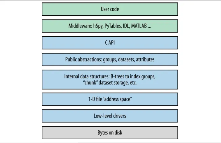
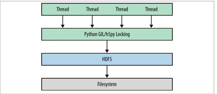
Before we jump into Python code examples, it’s useful to take a few minutes to address how HDF5 itself is organized. Figure 2-1 shows a cartoon of the various logical layers involved when using HDF5. Layers shaded in blue are internal to the library itself; layers in green represent software that uses HDF5.
Most client code, including the Python packages h5py and PyTables, uses the native C API (HDF5 is itself written in C). As we saw in the introduction, the HDF5 data model consists of three main public abstractions: datasets (see Chapter 3), groups (see Chap‐ ter 5), and attributes (see Chapter 6)in addition to a system to represent types. The C API (and Python code on top of it) is designed to manipulate these objects.
HDF5 uses a variety of internal data structures to represent groups, datasets, and at‐ tributes. For example, groups have their entries indexed using structures called “B-trees,” which make retrieving and creating group members very fast, even when hundreds of thousands of objects are stored in a group (see “How Groups Are Actually Stored” on page 65). You’ll generally only care about these data structures when it comes to perfor‐ mance considerations. For example, when using chunked storage (see Chapter 4), it’s important to understand how data is actually organized on disk.
The next two layers have to do with how your data makes its way onto disk. HDF5 objects all live in a 1D logical address space, like in a regular file. However, there’s an extra layer between this space and the actual arrangement of bytes on disk. HDF5 drivers
take care of the mechanics of writing to disk, and in the process can do some amazing things.
Figure 2-1. The HDF5 library: blue represents components inside the HDF5 library; green represents “client” code that calls into HDF5; gray represents resources provided by the operating system.
For example, the HDF5 core driver lets you use files that live entirely in memory and are blazingly fast. The family driver lets you split a single file into regularly sized pieces. And the mpio driver lets you access the same file from multiple parallel processes, using the Message Passing Interface (MPI) library (“MPI and Parallel HDF5” on page 119). All of this is transparent to code that works at the higher level of groups, datasets, and attributes.
Setting Up
That’s enough background material for now. Let’s get started with Python! But which
Python?
Python 2 or Python 3?
Python 2.7, the most recent minor release in the Python series, will also be the last 2.X release. Although it will be updated with bug fixes for an extended period of time, new Python code development is now carried out exclusively on the 3.X line. The NumPy package, h5py, PyTables, and many other packages now support Python 3. While (in my opinion) it’s a little early to recommend that newcomers start with Python 3, the future is clear.
So at the moment, there are two major versions of Python widely deployed simultane‐ ously. Since most people in the Python community are used to Python 2, the examples in this book are also written for Python 2. For the most part, the differences are minor; for example, on Python 3, the syntax for print is print(foo), instead of print foo. Wherever incompatibilities are likely to occur (mainly with string types and certain dictionary-style methods), these will be noted in the text.
“Porting” code to Python 3 isn’t actually that hard; after all, it’s still Python. Some of the most valuable features in Python 3 are already present in Python 2.7. A free tool is also available (2to3) that can accomplish most of the mechanical changes, for example changing print statements to print() function calls. Check out the migration guide (and the 2to3 tool) at http://www.python.org.
Code Examples
To start with, most of the code examples will follow this form:
>>> a = 1.0 >>> print a
1.0
Or, since Python prints objects by default, an even simpler form:
>>> a
1.0
Lines starting with >>> represent input to Python (>>> being the default Python prompt); other lines represent output. Some of the longer examples, where the program output is not shown, omit the >>> in the interest of clarity.
Examples intended to be run from the command line will start with the Unix-style "$" prompt:
$ python --version Python 2.7.3
Finally, to avoid cluttering up the examples, most of the code snippets you’ll find here will assume that the following packages have been imported:
>>> import numpy as np # Provides array object and data type objects
>>> import h5py # Provides access to HDF5
NumPy
“NumPy” is the standard numerical-array package in the Python world. This book as‐ sumes that you have some experience with NumPy (and of course Python itself), in‐ cluding how to use array objects.
Even if you’ve used NumPy before, it’s worth reviewing a few basic facts about how arrays work. First, NumPy arrays all have a fixed data type or “dtype,” represented by
dtype objects. For example, let’s create a simple 10-element integer array:
>>> arr = np.arange(10) >>> arr
array([0, 1, 2, 3, 4, 5, 6, 7, 8, 9])
The data type of this array is given by arr.dtype:
>>> arr.dtype
dtype('int32')
These dtype objects are how NumPy communicates low-level information about the type of data in memory. For the case of our 10-element array of 4-byte integers (32-bit or “int32” in NumPy lingo), there is a chunk of memory somewhere 40 bytes long that holds the values 0 through 9. Other code that receives the arr object can inspect the dtype object to figure out what the memory contents represent.
The preceding example might print dtype('int64') on your system. All this means is that the default integer size available to Python is 64 bits long, instead of 32 bits.
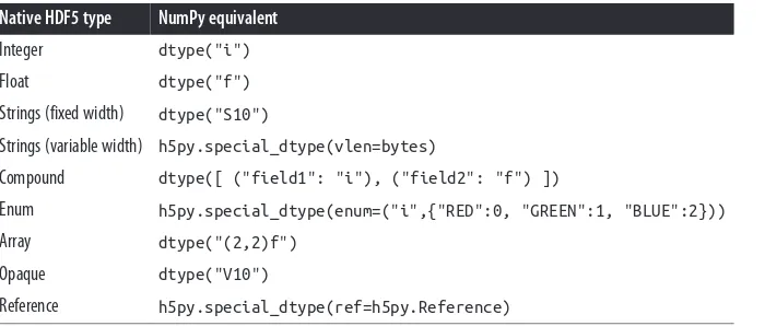
HDF5 uses a very similar type system; every “array” or dataset in an HDF5 file has a fixed type represented by a type object. The h5py package automatically maps the HDF5 type system onto NumPy dtypes, which among other things makes it easy to interchange data with NumPy. Chapter 3 goes into more detail about this process.
Slicing is another core feature of NumPy. This means accessing portions of a NumPy array. For example, to extract the first four elements of our array arr:
>>> out = arr[0:4] >>> out
array([0, 1, 2, 3])
You can also specify a “stride” or steps between points in the slice:
>>> out = arr[0:4:2] >>> out
array([0, 2])
In the NumPy world, slicing is implemented in a clever way, which generally creates arrays that refer to the data in the original array, rather than independent copies. For example, the preceding out object is likely a “view” onto the original arr array. We can test this:
>>> out[:] = 42 >>> out
array([42, 42]) >>> arr
array([42, 1, 42, 3, 4, 5, 6, 7, 8, 9])
This means slicing is generally a very fast operation. But you should be careful to ex‐ plicitly create a copy if you want to modify the resulting array without your changes finding their way back to the original:
>>> out2 = arr[0:4:2].copy()
Forgetting to make a copy before modifying a “slice” of the array is a very common mistake, especially for people used to environments like IDL. If you’re new to NumPy, be careful!
As we’ll see later, thankfully this doesn’t apply to slices read from HDF5 datasets. When you read from the file, since the data is on disk, you will always get a copy.
HDF5 and h5py
We’ll use the “h5py” package to talk to HDF5. This package contains high-level wrappers for the HDF5 objects of files, groups, datasets, and attributes, as well as extensive low-level wrappers for the HDF5 C data structures and functions. The examples in this book assume h5py version 2.2.0 or later, which you can get at http://www.h5py.org.
You should note that h5py is not the only commonly used package for talking to HDF5. PyTables is a scientific database package based on HDF5 that adds dataset indexing and an additional type system. Since we’ll be talking about native HDF5 constructs, we’ll stick to h5py, but I strongly recommend you also check out PyTables if those features interest you.
If you’re on Linux, it’s generally a good idea to install the HDF5 library via your package manager. On Windows, you can download an installer from http://www.h5py.org, or use one of the many distributions of Python that include HDF5/h5py, such as PythonXY, Anaconda from Continuum Analytics, or Enthought Python Distribution.
IPython
Apart from NumPy and h5py/HDF5 itself, IPython is a must-have component if you’ll be doing extensive analysis or development with Python. At its most basic, IPython is
a replacement interpreter shell that adds features like command history and Tab-completion for object attributes. It also has tons of additional features for parallel pro‐ cessing, MATLAB-style “notebook” display of graphs, and more.
The best way to explore the features in this book is with an IPython prompt open, following along with the examples. Tab-completion alone is worth it, because it lets you quickly see the attributes of modules and objects. The h5py package is specifically de‐ signed to be “explorable” in this sense. For example, if you want to discover what prop‐ erties and methods exist on the File object (see “Your First HDF5 File” on page 17), type h5py.File. and bang the Tab key:
>>> h5py.File.<TAB>
h5py.File.attrs h5py.File.get h5py.File.name h5py.File.close h5py.File.id h5py.File.parent h5py.File.copy h5py.File.items h5py.File.ref
h5py.File.create_dataset h5py.File.iteritems h5py.File.require_dataset h5py.File.create_group h5py.File.iterkeys h5py.File.require_group h5py.File.driver h5py.File.itervalues h5py.File.userblock_size h5py.File.fid h5py.File.keys h5py.File.values
h5py.File.file h5py.File.libver h5py.File.visit h5py.File.filename h5py.File.mode h5py.File.visititems h5py.File.flush h5py.File.mro
To get more information on a property or method, use ? after its name:
>>> h5py.File.close?
Type: instancemethod
Base Class: <type 'instancemethod'> String Form:<unbound method File.close> Namespace: Interactive
File: /usr/local/lib/python2.7/dist-packages/h5py/_hl/files.py Definition: h5py.File.close(self)
Docstring: Close the file. All open objects become invalid
By default, IPython will save the output of your statements in special hidden variables. This is generally OK, but can be surprising if it hangs on to an HDF5 object you thought was discarded, or a big array that eats up memory. You can turn this off by setting the IPython config‐ uration value cache_size to 0. See the docs at http://ipython.org for more information.
Timing and Optimization
For performance testing, we’ll use the timeit module that ships with Python. Examples using timeit will assume the following import:
The timeit function takes a (string or callable) command to execute, and an optional number of times it should be run. It then prints the total time spent running the com‐ mand. For example, if we execute the “wait” function time.sleep five times:
>>> import time
>>> timeit("time.sleep(0.1)", number=5) 0.49967818316434887
If you’re using IPython, there’s a similar built-in “magic” function called %timeit that runs the specified statement a few times, and reports the lowest execution time:
>>> %timeit time.sleep(0.1)
10 loops, best of 3: 100 ms per loop
We’ll stick with the regular timeit function in this book, in part because it’s provided by the Python standard library.
Since people using HDF5 generally deal with large datasets, performance is always a concern. But you’ll notice that optimization and benchmarking discussions in this book don’t go into great detail about things like cache hits, data conversion rates, and so forth. The design of the h5py package, which this book uses, leaves nearly all of that to HDF5. This way, you benefit from the hundreds of man years of work spent on tuning HDF5 to provide the highest performance possible.
As an application builder, the best thing you can do for performance is to use the API in a sensible way and let HDF5 do its job. Here are some suggestions:
1. Don’t optimize anything unless there’s a demonstrated performance problem. Then, carefully isolate the misbehaving parts of the code before changing anything.
2. Start with simple, straightforward code that takes advantage of the API features. For example, to iterate over all objects in a file, use the Visitor feature of HDF5 (see “Multilevel Iteration with the Visitor Pattern” on page 68) rather than cobbling to‐ gether your own approach.
3. Do “algorithmic” improvements first. For example, when writing to a dataset (see Chapter 3), write data in reasonably sized blocks instead of point by point. This lets HDF5 use the filesystem in an intelligent way.
4. Make sure you’re using the right data types. For example, if you’re running a compute-intensive program that loads floating-point data from a file, make sure that you’re not accidentally using double-precision floats in a calculation where single precision would do.
5. Finally, don’t hesitate to ask for help on the h5py or NumPy/Scipy mailing lists, Stack Overflow, or other community sites. Lots of people are using NumPy and HDF5 these days, and many performance problems have known solutions. The Python community is very welcoming.
The HDF5 Tools
We’ll be creating a number of files in later chapters, and it’s nice to have an independent way of seeing what they contain. It’s also a good idea to inspect files you create profes‐ sionally, especially if you’ll be using them for archiving or sharing them with colleagues. The earlier you can detect the use of an incorrect data type, for example, the better off you and other users will be.
HDFView
HDFView is a free graphical browser for HDF5 files provided by the HDF Group. It’s a little basic, but is written in Java and therefore available on Windows, Linux, and Mac. There’s a built-in spreadsheet-like browser for data, and basic plotting capabilities.
Figure 2-2. HDFView
Figure 2-2 shows the contents of an HDF5 file with multiple groups in the left-hand pane. One group (named “1”) is open, showing the datasets it contains; likewise, one dataset is opened, with its contents displayed in the grid view to the right.
ViTables
Figure 2-3 shows the same HDF5 file open in ViTables, another free graphical browser. It’s optimized for dealing with PyTables files, although it can handle generic HDF5 files perfectly well. One major advantage of ViTables is that it comes preinstalled with such Python distributions as PythonXY, so you may already have it.
Figure 2-3. ViTables
Command Line Tools
If you’re used to the command line, it’s definitely worth installing the HDF command-line tools. These are generally available through a package manager; if not, you can get them at www.hdfgroup.org. Windows versions are also available.
The program we’ll be using most in this book is called h5ls, which as the name suggests lists the contents of a file. Here’s an example, in which h5ls is applied to a file containing a couple of datasets and a group:
$ h5ls demo.hdf5
array Dataset {10} group Group
scalar Dataset {SCALAR}
We can get a little more useful information by using the option combo -vlr, which prints extended information and also recursively enters groups:
$ h5ls -vlr demo.hdf5
Storage: 40 logical bytes, 40 allocated bytes, 100.00% utilization Type: native int
Storage: 16 logical bytes, 16 allocated bytes, 100.00% utilization Type: native int
/scalar Dataset {SCALAR} Location: 1:800
Links: 1
Storage: 4 logical bytes, 4 allocated bytes, 100.00% utilization Type: native int
That’s a little more useful. We can see that the object at /array is of type “native int,” and is a 1D array 10 elements long. Likewise, there’s a dataset inside the group named group that is 2D, also of type native int.
h5ls is great for inspecting metadata like this. There’s also a program called h5dump, which prints data as well, although in a more verbose format:
DATASPACE SCALAR DATA {
(0): 42 } } } }
Your First HDF5 File
Before we get to groups and datasets, let’s start by exploring some of the capabilities of the File object, which will be your entry point into the world of HDF5.
Here’s the simplest possible program that uses HDF5:
>>> f = h5py.File("name.hdf5") >>> f.close()
The File object is your starting point; it has methods that let you create new datasets or groups in the file, as well as more pedestrian properties such as .filename and .mode.
Speaking of .mode, HDF5 files support the same kind of read/write modes as regular Python files:
>>> f = h5py.File("name.hdf5", "w") # New file overwriting any existing file
>>> f = h5py.File("name.hdf5", "r") # Open read-only (must exist)
>>> f = h5py.File("name.hdf5", "r+") # Open read-write (must exist)
>>> f = h5py.File("name.hdf5", "a") # Open read-write (create if doesn't exist)
There’s one additional HDF5-specific mode, which can save your bacon should you accidentally try to overwrite an existing file:
>>> f = h5py.File("name.hdf5", "w-")
This will create a new file, but fail if a file of the same name already exists. For example, if you’re performing a long-running calculation and don’t want to risk overwriting your output file should the script be run twice, you could open the file in w- mode:
>>> f = h5py.File("important_file.hdf5", "w-") >>> f.close()
>>> f = h5py.File("important_file.hdf5", "w-")
IOError: unable to create file (File accessability: Unable to open file)
By the way, you’re free to use Unicode filenames! Just supply a normal Unicode string and it will transparently work, assuming the underlying operating system supports the UTF-8 encoding:
>>> name = u"name_eta_\u03b7"
>>> f = h5py.File(name) >>> print f.filename
name_eta_η
You might wonder what happens if your program crashes with open files. If the program exits with a Python exception, don’t worry! The HDF library will automatically close every open file for you when the application exits.
Use as a Context Manager
One of the coolest features introduced in Python 2.6 is support for context managers. These are objects with a few special methods called on entry and exit from a block of code, using the with statement. The classic example is the built-in Python file object:
>>> with open("somefile.txt", "w") as f: ... f.write("Hello!")
The preceding code opens a brand-new file object, which is available in the code block with the name f. When the block exits, the file is automatically closed (even if an ex‐ ception occurs!).
The h5py.File object supports exactly this kind of use. It’s a great way to make sure the file is always properly closed, without wrapping everything in try/except blocks:
>>> with h5py.File("name.hdf5", "w") as f: ... print f["missing_dataset"]
KeyError: "unable to open object (Symbol table: Can't open object)" >>> print f
<Closed HDF5 file>
File Drivers
File drivers sit between the filesystem and the higher-level world of HDF5 groups, da‐ tasets, and attributes. They deal with the mechanics of mapping the HDF5 “address space” to an arrangement of bytes on disk. Typically you won’t have to worry about which driver is in use, as the default driver works well for most applications.
The great thing about drivers is that once the file is opened, they’re totally transparent. You just use the HDF5 library as normal, and the driver takes care of the storage me‐ chanics.
Here are a couple of the more interesting ones, which can be helpful for unusual prob‐ lems.
core driver
>>> f = h5py.File("name.hdf5", driver="core")
You can also tell HDF5 to create an on-disk “backing store” file, to which the file image is saved when closed:
>>> f = h5py.File("name.hdf5", driver="core", backing_store=True)
By the way, the backing_store keyword will also tell HDF5 to load any existing image from disk when you open the file. So if the entire file will fit in memory, you need to read and write the image only once; things like dataset reads and writes, attribute cre‐ ation, and so on, don’t take any disk I/O at all.
family driver
Sometimes it’s convenient to split a file up into multiple images, all of which share a certain maximum size. This feature was originally implemented to support filesystems that couldn’t handle file sizes above 2GB.
>>> # Split the file into 1-GB chunks
>>> f = h5py.File("family.hdf5", driver="family", memb_size=1024**3)
The default for memb_size is 231-1, in keeping with the historical origins of the driver.
mpio driver
This driver is the heart of Parallel HDF5. It lets you access the same file from multiple processes at the same time. You can have dozens or even hundreds of parallel computing processes, all of which share a consistent view of a single file on disk.
Using the mpio driver correctly can be tricky. Chapter 9 covers both the details of this driver and best practices for using HDF5 in a parallel environment.
The User Block
One interesting feature of HDF5 is that files may be preceeded by arbitrary user data. When a file is opened, the library looks for the HDF5 header at the beginning of the file, then 512 bytes in, then 1024, and so on in powers of 2. Such space at the beginning of the file is called the “user block,” and you can store whatever data you want there.
The only restrictions are on the size of the block (powers of 2, and at least 512), and that you shouldn’t have the file open in HDF5 when writing to the user block. Here’s an example:
>>> f = h5py.File("userblock.hdf5", "w", userblock_size=512) >>> f.userblock_size # Would be 0 if no user block present 512
>>> f.close()
>>> with open("userblock.hdf5", "rb+") as f: # Open as regular Python file
... f.write("a"*512)
CHAPTER 3
Working with Datasets
Datasets are the central feature of HDF5. You can think of them as NumPy arrays that live on disk. Every dataset in HDF5 has a name, a type, and a shape, and supports random access. Unlike the built-in np.save and friends, there’s no need to read and write the entire array as a block; you can use the standard NumPy syntax for slicing to read and write just the parts you want.
Dataset Basics
First, let’s create a file so we have somewhere to store our datasets:
>>> f = h5py.File("testfile.hdf5")
Every dataset in an HDF5 file has a name. Let’s see what happens if we just assign a new NumPy array to a name in the file:
>>> arr = np.ones((5,2)) >>> f["my dataset"] = arr
>>> dset = f["my dataset"] >>> dset
<HDF5 dataset "my dataset": shape (5, 2), type "<f8">
We put in a NumPy array but got back something else: an instance of the class h5py.Dataset. This is a “proxy” object that lets you read and write to the underlying HDF5 dataset on disk.
Type and Shape
Let’s explore the Dataset object. If you’re using IPython, type dset. and hit Tab to see the object’s attributes; otherwise, do dir(dset). There are a lot, but a few stand out:
>>> dset.dtype
Each dataset has a fixed type that is defined when it’s created and can never be changed. HDF5 has a vast, expressive type mechanism that can easily handle the built-in NumPy types, with few exceptions. For this reason, h5py always expresses the type of a dataset using standard NumPy dtype objects.
There’s another familiar attribute:
>>> dset.shape
(5, 2)
A dataset’s shape is also defined when it’s created, although as we’ll see later, it can be changed. Like NumPy arrays, HDF5 datasets can have between zero axes (scalar, shape ()) and 32 axes. Dataset axes can be up to 263-1 elements long.
Reading and Writing
Datasets wouldn’t be that useful if we couldn’t get at the underlying data. First, let’s see what happens if we just read the entire dataset:
>>> out = dset[...] >>> out
array([[ 1., 1.], [ 1., 1.], [ 1., 1.], [ 1., 1.], [ 1., 1.]]) >>> type(out)
<type 'numpy.ndarray'>
Slicing into a Dataset object returns a NumPy array. Keep in mind what’s actually hap‐ pening when you do this: h5py translates your slicing selection into a portion of the dataset and has HDF5 read the data from disk. In other words, ignoring caching, a slicing operation results in a read or write to disk.
Let’s try updating just a portion of the dataset:
>>> dset[1:4,1] = 2.0 >>> dset[...]
array([[ 1., 1.], [ 1., 2.], [ 1., 2.], [ 1., 2.], [ 1., 1.]])
Because Dataset objects are so similar to NumPy arrays, you may be tempted to mix them in with computational code. This may work for a while, but generally causes performance problems as the data is on disk instead of in memory.
Creating Empty Datasets
You don’t need to have a NumPy array at the ready to create a dataset. The method create_dataset on our File object can create empty datasets from a shape and type, or even just a shape (in which case the type will be np.float32, native single-precision float):
>>> dset = f.create_dataset("test1", (10, 10)) >>> dset
<HDF5 dataset "test1": shape (10, 10), type "<f4">
>>> dset = f.create_dataset("test2", (10, 10), dtype=np.complex64) >>> dset
<HDF5 dataset "test2": shape (10, 10), type "<c8">
HDF5 is smart enough to only allocate as much space on disk as it actually needs to store the data you write. Here’s an example: suppose you want to create a 1D dataset that can hold 4 gigabytes worth of data samples from a long-running experiment:
>>> dset = f.create_dataset("big dataset", (1024**3,), dtype=np.float32)
Now write some data to it. To be fair, we also ask HDF5 to flush its buffers and actually write to disk:
>>> dset[0:1024] = np.arange(1024) >>> f.flush()
Looking at the file size on disk:
$ ls -lh testfile.hdf5
-rw-r--r-- 1 computer computer 66K Mar 6 21:23 testfile.hdf5
Saving Space with Explicit Storage Types
When it comes to types, a few seconds of thought can save you a lot of disk space and also reduce your I/O time. The create_dataset method can accept almost any NumPy dtype for the underlying dataset, and crucially, it doesn’t have to exactly match the type of data you later write to the dataset.
Here’s an example: one common use for HDF5 is to store numerical floating-point data —for example, time series from digitizers, stock prices, computer simulations—any‐ where it’s necessary to represent “real-world” numbers that aren’t integers.
Often, to keep the accuracy of calculations high, 8-byte double-precision numbers will be used in memory (NumPy dtype float64), to minimize the effects of rounding error.
However, it’s common practice to store these data points on disk as single-precision, 4-byte numbers (float32), saving a factor of 2 in file size.
Let’s suppose we have such a NumPy array called bigdata:
>>> bigdata = np.ones((100,1000)) >>> bigdata.dtype
dtype('float64') >>> bigdata.shape
(100, 1000)
We could store this in a file by simple assignment, resulting in a double-precision dataset:
>>> with h5py.File('big1.hdf5','w') as f1: ... f1['big'] = bigdata
$ ls -lh big1.hdf5
-rw-r--r-- 1 computer computer 784K Apr 13 14:40 foo.hdf5
Or we could request that HDF5 store it as single-precision data:
>>> with h5py.File('big2.hdf5','w') as f2:
... f2.create_dataset('big', data=bigdata, dtype=np.float32)
$ ls -lh big2.hdf5
-rw-r--r-- 1 computer computer 393K Apr 13 14:42 foo.hdf5
Keep in mind that whichever one you choose, your data will emerge from the file in that format:
>>> f1 = h5py.File("big1.hdf5") >>> f2 = h5py.File("big2.hdf5") >>> f1['big'].dtype
dtype('float64') >>> f2['big'].dtype
dtype('float32')
Automatic Type Conversion and Direct Reads
But exactly how and when does the data get converted between the double-precision float64 in memory and the single-precision float32 in the file? This question is im‐ portant for performance; after all, if you have a dataset that takes up 90% of the memory in your computer and you need to make a copy before storing it, there are going to be problems.
But what if we want to go the other direction? Suppose we have a single-precision float dataset on disk, and want to read it in as double precision? There are a couple of reasons this might be useful. The result might be very large, and we might not have the memory space to hold both single- and double-precision versions in Python while we do the conversion. Or we might want to do the type conversion on the fly while reading from disk, to reduce the application’s runtime.
For big arrays, the best approach is to read directly into a preallocated NumPy array of the desired type. Let’s say we have the single-precision dataset from the previous ex‐ ample, and we want to read it in as double precision:
>>> dset = f2['big'] >>> dset.dtype
dtype('float32') >>> dset.shape
(100, 1000)
We allocate our new double-precision array on the Python side:
>>> big_out = np.empty((100, 1000), dtype=np.float64)
Here np.empty creates the array, but unlike np.zeros or np.ones it doesn’t bother to initialize the array elements. Now we request that HDF5 read directly into our output array:
>>> dset.read_direct(big_out)
That’s it! HDF5 fills up the empty array with the requested data. No extra arrays or time spent converting.
When using read_direct, you don’t always have to read the whole dataset. See “Reading Directly into an Existing Array” on page 34 for details.
Reading with astype
You may not always want to go through the whole rigamarole of creating a destination array and passing it to read_direct. Another way to tell HDF5 what type you want is by using the Dataset.astype context manager.
Let’s suppose we want to read the first 1000 elements of our “big” dataset in the previous example, and have HDF5 itself convert them from single to double precision:
>>> with dset.astype('float64'): ... out = dset[0,:]
>>> out.dtype
dtype('float64')
Finally, here are some tips to keep in mind when using HDF5’s automatic type conver‐ sion. They apply both to reads with read_direct or astype and also to writing data from NumPy into existing datasets:
1. Generally, you can only convert between types of the same “flavor.” For example, you can convert integers to floats, and floats to other floats, but not strings to floats or integers. You’ll get an unhelpful-looking IOError if you try.
2. When you’re converting to a “smaller” type (float64 to float32, or "S10" to "S5"), HDF5 will truncate or “clip” the values:
>>> f.create_dataset('x', data=1e256, dtype=np.float64) >>> print f['x'][...]
1e+256
>>> f.create_dataset('y', data=1e256, dtype=np.float32) >>> print f['y'][...]
inf
There’s no warning when this happens, so it’s in your interest to keep track of the types involved.
Reshaping an Existing Array
There’s one more trick up our sleeve with create_dataset, although this one’s a little more esoteric. You’ll recall that it takes a “shape” argument as well as a dtype argument. As long as the total number of elements match, you can specify a shape different from the shape of your input array.
Let’s suppose we have an array that stores 100 640×480-pixel images, stored as 640-element “scanlines”:
>>> imagedata.shape
(100, 480, 640)
Now suppose that we want to store each image as a “top half ” and “bottom half ” without needing to do the slicing when we read. When we go to create the dataset, we simply specify the new shape:
>>> f.create_dataset('newshape', data=imagedata, shape=(100, 2, 240, 640)) There’s no performance penalty. Like the built-in np.reshape, only the indices are shuffled around.
Fill Values
If you create a brand-new dataset, you’ll notice that by default it’s zero filled:
array([[0, 0], [0, 0]])
For some applications, it’s nice to pick a default value other than 0. You might want to set unmodified elements to -1, or even NaN for floating-point datasets.
HDF5 addresses this with a fill value, which is the value returned for the areas of a dataset that haven’t been written to. Fill values are handled when data is read, so they don’t cost you anything in terms of storage space. They’re defined when the dataset is created, and can’t be changed:
>>> dset = f.create_dataset('filled', (2,2), dtype=np.int32, fillvalue=42) >>> dset[...]
array([[42, 42], [42, 42]])
A dataset’s fill value is available on the fillvalue property:
>>> dset.fillvalue
42
Reading and Writing Data
Your main day-to-day interaction with Dataset objects will look a lot like your inter‐ actions with NumPy arrays. One of the design goals for the h5py package was to “recycle” as many NumPy metaphors as possible for datasets, so that you can interact with them in a familiar way.
Even if you’re an experienced NumPy user, don’t skip this section! There are important performance differences and implementation subtleties between the two that may trip you up.
Before we dive into the nuts and bolts of reading from and writing to datasets, it’s important to spend a few minutes discussing how Dataset objects aren’t like NumPy arrays, especially from a performance perspective.
Using Slicing Effectively
In order to use Dataset objects efficiently, we have to know a little about what goes on behind the scenes. Let’s take the example of reading from an existing dataset. Suppose we have the (100, 1000)-shape array from the previous example:
>>> dset = f2['big'] >>> dset
<HDF5 dataset "big": shape (100, 1000), type "<f4">
Now we request a slice:
>>> out = dset[0:10, 20:70] >>> out.shape
(10, 50)
Here’s what happens behind the scenes when we do the slicing operation:
1. h5py figures out the shape (10, 50) of the resulting array object.
2. An empty NumPy array is allocated of shape (10, 50). 3. HDF5 selects the appropriate part of the dataset.
4. HDF5 copies data from the dataset into the empty NumPy array.
5. The newly filled in NumPy array is returned.
You’ll notice that this implies a certain amount of overhead. Not only do we create a new NumPy array for each slice requested, but we have to figure out what size the array object should be, check that the selection falls within the bounds of the dataset, and have HDF5 perform the selection, all before we’ve read a single byte of data.
This leads us to the first and most important performance tip when using datasets: take reasonably sized slices.
Here’s an example: using our (100, 1000)-shape dataset, which of the following do you think is likely to be faster?
# Check for negative values and clip to 0
for ix in xrange(100):
for iy in xrange(1000):
val = dset[ix,iy] # Read one element
if val < 0: dset[ix, iy] = 0 # Clip to 0 if needed
or
# Check for negative values and clip to 0
for ix in xrange(100):
val = dset[ix,:] # Read one row
val[ val < 0 ] = 0 # Clip negative values to 0
dset[ix,:] = val # Write row back out
In the first case, we perform 100,000 slicing operations. In the second, we perform only 100.
This may seem like a trivial example, but the first example creeps into real-world code frequently; using fast in-memory slices on NumPy arrays, it is actually reasonably quick on modern machines. But once you start going through the whole slice-allocate-HDF5-read pipeline outlined here, things start to bog down.
The same applies to writing, although fewer steps are involved. When you perform a write operation, for example:
The following steps take place:
1. h5py figures out the size of the selection, and determines whether it is compatible with the size of the array being assigned.
2. HDF5 makes an appropriately sized selection on the dataset. 3. HDF5 reads from the input array and writes to the file.
All of the overhead involved in figuring out the slice sizes and so on, still applies. Writing to a dataset one element at a time, or even a few elements at a time, is a great way to get poor performance.
Start-Stop-Step Indexing
h5py uses a subset of the plain-vanilla slicing available in NumPy. This is the most familiar form, consisting of up to three indices providing a start, stop, and step.
For example, let’s create a simple 10-element dataset with increasing values:
>>> dset = f.create_dataset('range', data=np.arange(10)) >>> dset[...]
array([0, 1, 2, 3, 4, 5, 6, 7, 8, 9])
One index picks a particular element:
>>> dset[4] 4
Two indices specify a range, ending just before the last index:
>>> dset[4:8] array([4,5,6,7])
Three indices provide a “step,” or pitch, telling how many elements to skip:
>>> dset[4:8:2] array([4,6])
And of course you can get all the points by simply providing :, like this:
>>> dset[:]
array([0,1,2,3,4,5,6,7,8,9])
Like NumPy, you are allowed to use negative numbers to “count back” from the end of the dataset, with -1 referring to the last element:
>>> dset[4:-1] array([4,5,6,7,8])
Unlike NumPy, you can’t pull fancy tricks with the indices. For example, the traditional way to reverse an array in NumPy is this:
>>> a = np.arange(10) >>> a
array([0, 1, 2, 3, 4, 5, 6, 7, 8, 9]) >>> a[::-1]
array([9, 8, 7, 6, 5, 4, 3, 2, 1, 0])
But if you try it on a dataset, you get the following:
>>> dset[::-1]
ValueError: Step must be >= 1 (got -1)
Multidimensional and Scalar Slicing
By now you’ve gotten used to seeing the expression “...,” which is used as a slice in examples. This object has the built-in name Ellipsis in the Python world. You can use it as a “stand-in” for axes you don’t want to bother specifying:
>>> dset = f.create_dataset('4d', shape=(100, 80, 50, 20)) >>> dset[0,...,0].shape
(80, 50)
And of course you can get the entire contents by using Ellipsis by itself:
>>> dset[...].shape
(100, 80, 50, 20)
There is one oddity we should discuss, which is that of scalar datasets. In NumPy, there are two flavors of array containing one element. The first has shape (1,), and is an ordinary one-dimensional array. You can get at the value inside by slicing or simple indexing:
>>> dset = f.create_dataset('1d', shape=(1,), data=42) >>> dset.shape
(1,) >>> dset[0] 42
>>> dset[...] array([42])
Note, by the way, how using Ellipsis provides an array with one element, whereas integer indexing provides the element itself.
The second flavor has shape () (an empty tuple) and can’t be accessed by indexing:
>>> dset = f.create_dataset('0d', data=42) >>> dset.shape
()
>>> dset[0]
ValueError: Illegal slicing argument for scalar dataspace >>> dset[...]
array(42)