Python Geospatial Development Essentials Utilize Python with open source libraries to build a lightweight, portable, and customizable GIS desktop application pdf pdf

(1)

(2)

Python Geospatial

Development Essentials

Utilize Python with open source libraries to

build a lightweight, portable, and customizable

GIS desktop application

Karim Bahgat

BIRMINGHAM - MUMBAI

(3)

Python Geospatial Development Essentials

Copyright © 2015 Packt Publishing

All rights reserved. No part of this book may be reproduced, stored in a retrieval

system, or transmitted in any form or by any means, without the prior written

permission of the publisher, except in the case of brief quotations embedded in

critical articles or reviews.

Every effort has been made in the preparation of this book to ensure the accuracy

of the information presented. However, the information contained in this book is

sold without warranty, either express or implied. Neither the author, nor Packt

Publishing, and its dealers and distributors will be held liable for any damages

caused or alleged to be caused directly or indirectly by this book.

Packt Publishing has endeavored to provide trademark information about all of the

companies and products mentioned in this book by the appropriate use of capitals.

However, Packt Publishing cannot guarantee the accuracy of this information.

First published: June 2015

Production reference: 1100615

Published by Packt Publishing Ltd.

Livery Place

35 Livery Street

Birmingham B3 2PB, UK.

ISBN 978-1-78217-540-7

(4)

Credits

Author

Karim Bahgat

Reviewers

Gregory Giuliani

Jorge Samuel Mendes de Jesus Athanasios Tom Kralidis John Maurer

Adrian Vu

Commissioning Editor

Amarabha Banerjee

Acquisition Editors

Larissa Pinto Rebecca Youé

Content Development Editor

Merwyn D'souza

Technical Editor

Prajakta Mhatre

Copy Editor

Charlotte Carneiro

Project Coordinator

Neha Bhatnagar

Proofreader Safis Editing

Indexer

Rekha Nair

Production Coordinator

Manu Joseph

Cover Work

Manu Joseph

(5)

About the Author

Karim Bahgat

holds an MA in peace and conflict transformation from the

University of Tromsø in Norway, where he focused on the use of geographic

information systems (GIS), opinion survey data, and open source programming

tools in conflict studies. Since then, he has been employed as a research assistant

for technical and geospatial work at the Peace Research Institute Oslo (PRIO)

and the International Law and Policy Institute (ILPI). Karim was part of the early

prototyping of the PRIO-GRID unified spatial data structure for social science and

conflict research, and is currently helping develop a new updated version (

https:// www.prio.org/Data/PRIO-GRID/

).

His main use of technology, as a developer, has been with Python programming,

geospatial tools and mapping, the geocoding of textual data, data visualization,

application development, and some web technology. Karim is the author of a journal

article publication, numerous data- and GIS-oriented Python programming libraries,

the Easy Georeferencer free geocoding software, and several related technical

websites, including

www.pythongisresources.wordpress.com

.

I am very grateful for the detailed feedback, suggestions, and

troubleshooting of chapters from the reviewers; the encouragement

and guidance from the publisher's administrators and staff, and

the patience and encouragement from friends, family, colleagues,

and loved ones (especially my inspirational sidekicks, Laura and

Murdock). I also want to thank all my teachers at the Chapman

University and University of North Dakota, who got me here in the

first place. They helped me think out of the box and led me into this

(6)

About the Reviewers

Gregory Giuliani

is a geologist with a PhD in environmental sciences (theme:

spatial data infrastructure for the environment). He is a senior scientific associate at the

University of Geneva (Switzerland) and the focal point for spatial data infrastructure

(SDI) at GRID-Geneva. He is the manager of the EU/FP7 EOPOWER project and the

work package leader in the EU/FP7 enviroGRIDS and AfroMaison projects, where he

coordinates SDI development and implementation. He also participated in the EU/

FP7 ACQWA project and is the GRID-Geneva lead developer of the PREVIEW Global

Risk Data Platform (

http://preview.grid.unep.ch

). He coordinates and develops

capacity building material on SDI for enviroGRIDS and actively participates and

contributes to various activities of the Global Earth Observation System of Systems

(GEOSS). Specialized in OGC standards, interoperability, and brokering technology for

environmental data and services, he is the coordinator of the Task ID-02 "Developing

Institutional and Individual Capacity" for GEO/GEOSS.

Jorge Samuel Mendes de Jesus

has 15 years of programming experience in

the field of Geoinformatics, with a focus on Python programming, OGC web

services, and spatial databases.

He has a PhD in geography and sustainable development from Ben-Gurion University

of the Negev, Israel. He has been employed by the Joint Research Center (JRC), Italy,

where he worked on projects such as EuroGEOSS, Intamap, and Digital Observatory

for Protected Areas (DOPA). He continued his professional career at Plymouth

Marine Laboratory, UK, as a member of the Remote Sensing Group contributing to the

NETMAR project and actively promoting the implementation of the WSDL standard

in PyWPS. He currently works at ISRIC—World Soil Information in the Netherlands,

where he supports the development of Global Soil Information Facilities (GSIF).

(7)

Athanasios Tom Kralidis

is a senior systems scientist for the Meteorological

Service of Canada, where he provides geospatial technical and architectural

leadership in support of MSC's data. Tom's professional background includes key

involvement in the development and integration of geospatial standards, systems,

and services for the Canadian Geospatial Data Infrastructure (CGDI) with Natural

Resources Canada. He also uses these principles in architecting RésEau, Canada's

water information portal. Tom is the lead architect of the renewal of the World

Ozone and Ultraviolet Radiation Data Centre (WOUDC) in support of the WMO

Global Atmospheric Watch.

Tom is active in the Open Geospatial Consortium (OGC) community, and was

lead contributor to the OGC Web Map Context Documents Specification. He was

also a member of the CGDI Architecture Advisory Board, as well as part of the

Canadian Advisory Committee to ISO Technical Committee 211 Geographic

information/Geomatics.

Tom is a developer on the MapServer, GeoNode, QGIS, and OWSLib open source

software projects, and part of the MapServer Project Steering Committee. He

is the founder and lead developer of

pycsw

, an OGC-compliant CSW reference

implementation. Tom is a charter member of the Open Source Geospatial

Foundation. He holds a bachelor's degree in geography from York University,

a GIS certification from Algonquin College, and a master's degree in geography

and environmental studies (research and dissertation in geospatial web services/

infrastructure) from Carleton University. Tom is a certified Geomatics Specialist

(GIS/LIS) with the Canadian Institute of Geomatics.

John Maurer

is a programmer and data manager at the Pacific Islands Ocean

Observing System (PacIOOS) in Honolulu, Hawaii. He creates and configures

web interfaces and data services to provide access, visualization, and mapping of

oceanographic data from a variety of sources, including satellite remote sensing,

forecast models, GIS layers, and in situ observations (buoys, sensors, shark tracking,

and so on) throughout the insular Pacific. He obtained a graduate certificate in

(8)

Adrian Vu

is a web and mobile developer based in Singapore, and has over

10 years of experience working on various projects for start-ups and organizations.

He holds a BSc in information systems management (majoring in business

intelligence and analytics) from Singapore Management University. Occasionally, he

likes to dabble in new frameworks and technologies, developing many useful apps

for all to use and play with.

(9)

www.PacktPub.com

Support files, eBooks, discount offers, and more

For support files and downloads related to your book, please visit

www.PacktPub.com

.

Did you know that Packt offers eBook versions of every book published, with PDF

and ePub files available? You can upgrade to the eBook version at

www.PacktPub.com

and as a print book customer, you are entitled to a discount on the eBook copy. Get in

touch with us at

service@packtpub.com

for more details.

At

www.PacktPub.com

, you can also read a collection of free technical articles,

sign up for a range of free newsletters and receive exclusive discounts and offers

on Packt books and eBooks.

TM

https://www2.packtpub.com/books/subscription/packtlib

Do you need instant solutions to your IT questions? PacktLib is Packt's online digital

book library. Here, you can search, access, and read Packt's entire library of books.

Why subscribe?

• Fully searchable across every book published by Packt

• Copy and paste, print, and bookmark content

• On demand and accessible via a web browser

Free access for Packt account holders

(10)

[ i ]

Preface

Python has become the language of choice for many in the geospatial industry.

Some use Python as a way to automate their workflows in software, such as ArcGIS

or QGIS. Others play around with the nuts and bolts of Python's immense variety of

third-party open source geospatial toolkits.

Given all the programming tools available and the people already familiar with

geospatial software, there is no reason why you should have to choose either one or

the other. Programmers can now develop their own applications from scratch to better

suit their needs. Python is, after all, known as a language for rapid development.

By developing your own application, you can have fun with it, experiment with

new visual layouts and creative designs, create platforms for specialized workflows,

and tailor to the needs of others.

What this book covers

Chapter 1 ,

Preparing to Build Your Own GIS Application

, talks about the benefits

of developing a custom geospatial application and describes how to set up your

development environment, and create your application folder structure.

Chapter 2 ,

Accessing Geodata

, implements the crucial data loading and saving capabilities

of your application for both vector and raster data.

Chapter 3 ,

Designing the Visual Look of Our Application

, creates and puts together the

basic building blocks of your application's user interface, giving you a first look at

what your application will look like.

(15)

Chapter 5 ,

Managing and Organizing Geographic Data

, creates a basic functionality for

splitting, merging, and cleaning both the vector and raster data.

Chapter 6 ,

Analyzing Geographic Data

, develops basic analysis functionality, such as

overlay statistics, for vector and raster data.

Chapter 7 ,

Packaging and Distributing Your Application

, wraps it all up by showing you

how to share and distribute your application, so it is easier for you or others to use it.

Chapter 8 ,

Looking Forward

, considers how you may wish to proceed to further build

on, customize, and extend your basic application into something more elaborate or

specialized in whichever way you want.

What you need for this book

There are no real requirements for this book. However, to keep the book short and

sweet, the instructions assume that you have a Windows operating system. If you

are on Mac OS X or Linux, you should still be able create and run the application,

but then you will have to figure out the equivalent installation instructions for your

operating system. You may be forced to deal with compiling C++ code and face the

potential of unexpected errors. All other installations will be covered throughout the

book, including which Python version to use.

Who this book is for

This book is ideal for Python programmers and software developers who are tasked

with or wish to make a customizable special-purpose GIS application, or are interested

in expanding their knowledge of working with spatial data cleaning, analysis, or map

visualization. Analysts, political scientists, geographers, and GIS specialists seeking

a creative platform to experiment with cutting-edge spatial analysis, but are still

only beginners in Python, will also find this book beneficial. Familiarity with Tkinter

application development in Python is preferable but not mandatory.

Conventions

In this book, you will find a number of text styles that distinguish between different

(16)

[ vii ]

Code words in text, database table names, folder names, filenames, file extensions,

pathnames, dummy URLs, user input, and Twitter handles are shown as follows:

"Download the Shapely wheel file that fits our system, looking something like

Shapely-1.5.7-cp27-none-win32.whl

."

A block of code is set as follows:

class LayerGroup: def __init__(self): self.layers = list()

self.connected_maps = list() def __iter__(self):

for layer in self.layers: yield layer

def add_layer(self, layer): self.layers.append(layer)

def move_layer(self, from_pos, to_pos): layer = self.layers.pop(from_pos) self.layers.insert(to_pos, layer) def remove_layer(self, position): self.layers.pop(position) def get_position(self, layer): return self.layers.index(layer)

Any command-line input or output is written as follows:

>>> import PIL, PIL.Image

>>> img = PIL.Image.open("your/path/to/icon.png") >>> img.save("your/path/to/pythongis/app/icon.ico",

sizes=[(255,255),(128,128),(64,64),(48,48),(32,32),(16,16),(8,8)])

New terms

and

important words

are shown in bold. Words that you see on

the screen, for example, in menus or dialog boxes, appear in the text like this:

"Click on the

Inno Setup

link on the left side."

(17)

Tips and tricks appear like this.

Reader feedback

Feedback from our readers is always welcome. Let us know what you think about

this book—what you liked or disliked. Reader feedback is important for us as it helps

us develop titles that you will really get the most out of.

To send us general feedback, simply e-mail

feedback@packtpub.com

, and mention

the book's title in the subject of your message.

If there is a topic that you have expertise in and you are interested in either writing

or contributing to a book, see our author guide at

www.packtpub.com/authors

.

Customer support

Now that you are the proud owner of a Packt book, we have a number of things to

help you to get the most from your purchase.

Downloading the example code

You can download the example code files from your account at

http://www. packtpub.com

for all the Packt Publishing books you have purchased. If you

purchased this book elsewhere, you can visit

http://www.packtpub.com/support

and register to have the files e-mailed directly to you.

Errata

Although we have taken every care to ensure the accuracy of our content, mistakes do

happen. If you find a mistake in one of our books—maybe a mistake in the text or the

code—we would be grateful if you could report this to us. By doing so, you can save

If you find any errata, please report them by visiting

http://www.packtpub.com/ submit-errata

, selecting your book, clicking on the

Errata

Submission

Form

link,

and entering the details of your errata. Once your errata are verified, your submission

(18)

[ ix ]

To view the previously submitted errata, go to

https://www.packtpub.com/books/ content/support

and enter the name of the book in the search field. The required

information will appear under the

Errata

section.

Piracy

Piracy of copyrighted material on the Internet is an ongoing problem across all

media. At Packt, we take the protection of our copyright and licenses very seriously.

If you come across any illegal copies of our works in any form on the Internet, please

provide us with the location address or website name immediately so that we can

pursue a remedy.

Please contact us at

copyright@packtpub.com

with a link to the suspected

pirated material.

We appreciate your help in protecting our authors and our ability to bring you

valuable content.

Questions

(19)

(20)

[ 1 ]

Preparing to Build Your

Own GIS Application

You are here because you love Python programming and are interested in making

your own

Geographic Information Systems

(

GIS

) application. You want to create a

desktop application, in other words, a user interface, that helps you or others create,

process, analyze, and visualize geographic data. This book will be your step-by-step

guide toward that goal.

We assume that you are someone who enjoys programming and being creative but

are not necessarily a computer science guru, Python expert, or seasoned GIS analyst.

To successfully proceed with this book, it is recommended that you have a basic

introductory knowledge of Python programming that includes classes, methods,

and the

Tkinter

toolkit, as well as some core GIS concepts. If you are a newcomer to

some of these, we will still cover some of the basics, but you will need to have the

interest and ability to follow along at a fast pace.

In this introductory chapter, you will cover the following:

• Learn some of the benefits of creating a GIS application from scratch

• Set up your computer, so you can follow the book instructions.

• Become familiar with the roadmap toward creating our application.

Why reinvent the wheel?

The first step in preparing ourselves for this book is in convincing ourselves why we

want to make our own GIS application, as well as to be clear about our motives. Spatial

analysis and GIS have been popular for decades and there is plenty of GIS software

out there, so why go through the trouble of reinventing the wheel? Firstly, we aren't

really reinventing the wheel, since Python can be extended with plenty of third-party

libraries that take care of most of our geospatial needs (more on that later).

(21)

For me, the main motivation stems from the problem that most of today's GIS

applications are aimed at highly capable and technical users who are well-versed in

GIS or computer science, packed with a dizzying array of buttons and options that

will scare off many an analyst. We believe that there is a virtue in trying to create a

simpler and more user-friendly software for beginner GIS users or even the broader

public, without having to start completely from scratch. This way, we also add more

alternatives for users to choose from, as supplements to the current GIS market

dominated by a few major giants, notably ArcGIS and QGIS, but also others such as

GRASS, uDig, gvSIG, and more.

Another particularly exciting reason to create your own GIS from scratch is to make

your own domain-specific special purpose

software for any task you can imagine,

whether it is a water flow model GIS, an ecological migrations GIS, or even a GIS

for kids. Such specialized tasks that would usually require many arduous steps in

an ordinary GIS, could be greatly simplified into a single button and accompanied

(22)

[ 3 ]

Also, by creating your GIS from scratch, it is possible to have greater control of the

size and portability of your application. This can enable you to go small—letting your

application have faster startup time, and travel the Internet or on a USB-stick easily.

Although storage space itself is not as much of an issue these days, from a user's

perspective, installing a 200 MB application is still a greater psychological investment

with a greater toll in terms of willingness to try it than a mere 30 MB application (all

else being equal). This is particularly true in the realm of smartphones and tablets, a

very exciting market for special-purpose

geospatial apps. While the specific application

we make in this book will not be able to run on iOS or Android devices, it will run on

Windows 8-based hybrid tablets, and can be rebuilt around a different GUI toolkit in

order to support iOS or Android (we will mention some very brief suggestions for

this in

Chapter 8 ,

Looking Forward

).

Finally, the utility and philosophy of free and open source software may be an

important motivation for some of you. Many people today, learn to appreciate open

source GIS after losing access to subscription-based applications like ArcGIS when

they complete their university education or change their workplace. By developing

your own open source GIS application and sharing with others, you can contribute

back to and become part of the community that once helped you.

Setting up your computer

In this book, we follow steps on how to make an application that is developed

in a Windows environment. This does not mean that the application cannot be

developed on Mac OS X or Linux, but those platforms may have slightly different

installation instructions and may require compiling of the binary code that is outside

the scope of this book. Therefore, we leave that choice up to the reader. In this book,

which focuses on Windows, we avoid the problem of compiling it altogether, using

precompiled versions where possible (more on this later).

The development process itself will be done using Python 2.7, specifically the

32-bit version, though 64-bit can theoretically be used as well (note that this is the

bit version of your Python installation and has nothing to do with the bit version

of your operating system). Although there exists many newer versions, version 2.7

is the most widely supported in terms of being able to use third-party packages. It

has also been reported that the version 2.7 will continue to be actively developed and

promoted until the year 2020. It will still be possible to use after support has ended.

If you do not already have version 2.7, install it now, by following these steps:

1. Go to

https://www.python.org/

.

(23)

3. Download and run the installation program.

For the actual code writing and editing, we will be using the built-in

Python

Interactive Development Environment

(

IDLE

), but you may of course use any

code editor you want. The IDLE lets you write long scripts that can be saved to

files and offers an interactive shell window to execute one line at a time. There

should be a desktop or start-menu link to Python IDLE after installing Python.

Installing third-party packages

In order to make our application, we will have to rely on the rich and varied

ecosystem of third-party packages that already exists for GIS usage.

The Python Package Index (PyPI) website currently lists more than 240 packages tagged Topic :: Scientific/Engineering ::

GIS. For a less overwhelming overview of the more popular GIS-related Python libraries, check out the catalogue at the

Python-GIS-Resources website created by the author:

http://pythongisresources.wordpress.com/

We will have to define which packages to use and install, and this depends on

the type of application we are making. What we want to make in this book is a

lightweight, highly portable, extendable, and general-purpose GIS application.

For these reasons, we avoid heavy packages like GDAL, NumPy, Matplotlib, SciPy,

and Mapnik (weighing in at about 30 MB each or about 150-200 MB if we combine

them all together). Instead, we focus on lighter third-party packages specialized for

each specific functionality.

Dropping these heavy packages is a bold decision, as they contain a

lot of functionality, and are reliable, efficient, and a dependency for

many other packages. If you decide that you want to use them in an application where size is not an issue, you may want to begin now by installing the multipurpose NumPy and possibly SciPy, both of which

have easy-to-use installers from their official websites. The other heavy packages will be briefly revisited in later chapters.

Specific installation instructions are given for each package in the chapter where

(24)

[ 5 ] Chapter Installation Purpose

1 Python

1 PIL Raster data, management, and analysis 1 Shapely Vector management and analysis 2 PyShp Data

2 PyGeoj Data

2 Rtree Vector data speedup 4 PyAgg Visualization

7 Py2exe Application distribution

The typical way to install Python packages is using pip (included with Python 2.7), which downloads and installs packages directly from the Python Package Index website. Pip is used in the following way:

• Step 1—open your operating system's command line (not the Python IDLE). On Windows, this is done by searching your system for cmd.exe and running it.

• Step 2—in the black screen window that pops up, one simply types pip install packagename. This will only work if

pip is on your system's environment path. If this is not the case, a quick fix is to simply type the full path to the pip script

C:\Python27\Scripts\pip instead of just pip. For C or C++ based packages, it is becoming increasingly popular to make them available as precompiled wheel files ending in .whl, which has caused some confusion on how to install them. Luckily, we can use pip to install these wheel files as well, by simply

downloading the wheel and pointing pip to its file path.

Since some of our dependencies have multiple purposes and are not unique to just

one chapter, we will install these ones now. One of them is the

Python Imaging

Library

(

PIL

), which we will use for the raster data model and for visualization.

Let's go ahead and install PIL for Windows now:

1. Go to

https://pypi.python.org/pypi/Pillow/2.6.1

.

2. Click on the latest

.exe

file link for our 32-bit Python 2.7 environment

to download the PIL installer, which is currently

Pillow-2.6.1.win32-py2.7.exe

.

3. Run the installation file.

(25)

Another central package we will be using is Shapely, used for location testing and

geometric manipulation. To install it on Windows, perform the following steps:

1. Go to

http://www.lfd.uci.edu/~gohlke/pythonlibs/#shapely

.

2. Download the Shapely wheel file that fits our system, looking something like

Shapely-1.5.7-cp27-none-win32.whl

.

3. As described earlier, open a command line window and type

C:\Python27\ Scripts\pip install path\to\Shapely-1.5.7-cp27-none-win32.whl

to unpack the precompiled binaries.

4. To make sure it was installed correctly, open the IDLE interactive shell and

type

import shapely

.

Imagining the roadmap ahead

Before we begin developing our application, it is important that we create a vision

of how we want to structure our application. In Python terms, we will be creating

a multilevel package with various subpackages and submodules to take care of

different parts of our functionality, independently of any user interface. Only on top

of this underlying functionality do we create the visual user interface as a way to

access and run that underlying code. This way, we build a solid system, and allow

power-users to access all the same functionality via Python scripting for greater

automation and efficiency, as exists for ArcGIS and QGIS.

To setup the main Python package behind our application, create a new folder called

pythongis

anywhere on your computer. For Python to be able to interpret the folder

pythongis

as an importable package, it needs to find a file named

__init__.py

in

that folder. Perform the following steps:

1. Open

Python IDLE

from the Windows start menu.

2. The first window to pop up is the interactive shell. To open the script editing

window click on

File

and

New

.

3. Click on

File

and then

Save As

.

4. In the dialog window that pops up, browse into the

pythongis

folder,

type

__init__.py

as the filename, and click on

Save

.

(26)

[ 7 ]

For a more detailed introduction to the differences between vector and raster data, and other basic GIS concepts, we refer the reader to the book Learning Geospatial Analysis with Python, by Joel Lawhead.

You can find this book at:

https://www.packtpub.com/application-development/ learning-geospatial-analysis-python

Since vector and raster data are so fundamentally different in all regards, we split

our package in two, one for vector and one for raster. Using the same method as

earlier, we create two new subpackage folders within the

pythongis

package; one

called

vector

and one called

raster

(each with the same aforementioned empty

__init__.py

file). Thus, the structure of our package will look as follows (note that

: package

is not part of the folder name):

To make our new

vector

and

raster

subpackages importable by our top level

pythongis

package, we need to add the following relative import statements in

pythongis/__init__.py

:

from . import vector from . import raster

Throughout the course of this book, we will build the functionality of these two data

types as a set of Python modules in their respective folders. Eventually, we want to

end up with a GIS application that has only the most basic of geospatial tools so that

we will be able to load, save, manage, visualize, and overlay data, each of which will

be covered in the following chapters.

As far as our final product goes, since we focus on clarity and simplicity, we do not

put too much effort into making it fast or memory efficient. This comes from an often

repeated saying among programmers, an example of which is found in

Structured

Programming with go to Statements

, ACM, Computing Surveys 6 (4):

premature optimization is the root of all evil

(27)

This leaves us with software that works best with small files, which in most cases

is good enough. Once you have a working application and you feel that you need

support for larger or faster files, then it's up to you if you want to put in the extra

effort of optimization.

The GIS application you end up with at the end of the book is simple but functional,

and is meant to serve as a framework that you can easily build on. To leave you with

some ideas to pick up on, we placed various information boxes throughout the book

with ways that you can optimize or extend your application. For any of the core topics

and features that we were not able to cover earlier in the book, we give a broader

discussion of missing functionality and future suggestions in the final chapter.

Summary

In this chapter, you learned about why you want to create a GIS application using

Python, set up our programming environment, installed some recurring packages,

and created your application structure and framework.

In the next chapter, you will take the first step toward making a geospatial application,

(28)

[ 9 ]

Accessing Geodata

All GIS processing must start with geographic data, so we begin our application by

building the capacity to interact with, load, and save various geographic file formats.

This chapter is divided into a vector and raster section, and in each section, we will

cover the following:

• Firstly, we create a data interface which means understanding data structures

and how to interact with them.

• Secondly and thirdly, any format-specific differences are outsourced to

separate loader and saver modules.

This is a lot of functionality to fit into one chapter, but by working your way through,

you will learn a lot about data structures, and file formats, and end up with a solid

foundation for your application.

The approach

In our efforts to build data access in this chapter, we focus on simplicity,

understanding, and lightweight libraries. We create standardized data interfaces

for vector and raster data so that we can use the same methods and expect the same

results on any data, without worrying about file format differences. They are not

necessarily optimized for speed or memory efficiency as they load entire files into

memory at once.

In our choice of third-party libraries for loading and saving, we focus on

format-specific ones, so that we can pick and choose which formats to support and thus

maintain a lightweight application. This requires some more work but allows us

(29)

If the size is not an issue in your application, you may wish to instead use the more powerful GDAL library, which can single-handedly load and save a much wider range of both vector and raster formats. To use GDAL, I suggest downloading and installing a precompiled version from http://www.lfd.uci.edu/~gohlke/pythonlibs/#gdal. On top of GDAL, the packages Fiona (http://www.lfd.uci. edu/~gohlke/pythonlibs/#fiona) and Rasterio (http://www. lfd.uci.edu/~gohlke/pythonlibs/#rasterio) provide a more convenient and Pythonic interface to GDAL's functionality for vector and raster data, respectively.

Vector data

We begin by adding support for vector data. We will be creating three submodules

inside our

vector

package:

data

,

loader

, and

saver

. To make these accessible from

their parent vector package, we need to import it in

vector/__init__.py

as follows:

from . import data from . import loader from . import saver

A data interface for vector data

The first thing we want is

a data interface that we can conveniently interact with.

This data interface will be contained in a module of its own, so create this module

now and save it as

vector/data.py

.

We start off with a few basic imports, including compatibility functions for Shapely

(which we installed in

Chapter 1 ,

Preparing to Build Your Own GIS Application

) and the

spatial indexing abilities of

Rtree

, a package we will install later. Note that vector data

loading and saving, are handled by separate modules that we have not yet created,

but since they are accessed through our data interface, we need to import them here:

# import builtins

import sys, os, itertools, operator from collections import OrderedDict import datetime

# import shapely geometry compatibility functions # ...and rename them for clarity

import shapely

(30)

[ 11 ]

# import rtree for spatial indexing import rtree

# import internal modules from . import loader from . import saver

Downloading the example code

You can download the example code files from your account at

http://www.packtpub.com for all the Packt Publishing books you have purchased. If you purchased this book elsewhere, you can visit http://www.packtpub.com/support and register

to have the files e-mailed directly to you.

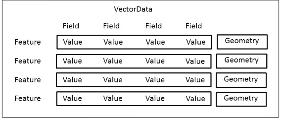
The vector data structure

Geographic vector data can be thought of as a table of data. Each row in the

table is an observation (say, a country), and holds one or more attributes, or piece

of information for that observation (say, population). In a vector data structure, rows

are known as a

features

, and have additional geometry definitions (coordinates that

define, say, the shape and location of a country). An overview of the structure may

therefore look something like this:

In our implementation of the vector data structure, we therefore create the interface

as a

VectorData

class. To create and populate a

VectorData

instance with data, we

can give it a

filepath

argument that it loads via the loader module that we create

later. We also allow for optional keyword arguments to pass to the loader, which

as we shall see includes the ability to specify text encoding. Alternatively, an empty

VectorData

instance can be created by not passing it any arguments. While creating

an empty instance, it is possible to specify the geometry type of the entire data instance

(meaning, it can only hold either polygon, line, or point geometries), otherwise it will

set the data type based on the geometry type of the first feature that is added.

(31)

In addition to storing the fieldnames and creating features from rows and geometries,

a

VectorData

instance remembers the

filepath

origin of the loaded data if applicable,

and the

Coordinate Reference System

(

CRS

) which defaults to unprojected WGS84 if

not specified.

To store the features, rather than using lists or dictionaries, we use an

ordered

dictionary that allows us to identify each feature with a unique ID, sort the

features, and perform fast and frequent feature lookups. To ensure that each

feature in

VectorData

has a unique ID, we define a unique ID generator and

attach independent ID generator instances to each

VectorData

instance.

To let us interact with the

VectorData

instance, we add various magic methods

to enable standard Python operations such as getting the number of features in the

data, looping through them, and getting and setting them through indexing their ID.

Finally, we include a convenient

add_feature

and

copy

method. Take a look at the

following code:

def ID_generator(): i = 0

while True: yield i i += 1 class VectorData:

def __init__(self, filepath=None, type=None, **kwargs): self.filepath = filepath

# type is optional and will make the features ensure that all geometries are of that type

# if None, type enforcement will be based on first geometry found

self.type = type

if filepath:

fields,rows,geometries,crs = loader.from_file(filepath, **kwargs) else:

fields,rows,geometries,crs = [],[],[],"+proj=longlat +ellps=WGS84 +datum=WGS84 +no_defs"

self.fields = fields

(32)

[ 13 ]

ids_rows_geoms =

itertools.izip(self._id_generator,rows,geometries)

featureobjs = (Feature(self,row,geom,id=id) for id,row,geom in ids_rows_geoms )

self.features = OrderedDict([ (feat.id,feat) for feat in featureobjs ])

self.crs = crs def __len__(self): """

How many features in data. """

return len(self.features) def __iter__(self):

"""

Loop through features in order. """

for feat in self.features.itervalues(): yield feat

def __getitem__(self, i): """

Get a Feature based on its feature id. """

if isinstance(i, slice):

raise Exception("Can only get one feature at a time") else:

return self.features[i] def __setitem__(self, i, feature): """

Set a Feature based on its feature id. """

if isinstance(i, slice):

raise Exception("Can only set one feature at a time") else:

self.features[i] = feature ### DATA ###

(33)

def copy(self):

new = VectorData()

new.fields = [field for field in self.fields]

featureobjs = (Feature(new, feat.row, feat.geometry) for feat in self )

new.features = OrderedDict([ (feat.id,feat) for feat in featureobjs ])

if hasattr(self, "spindex"): new.spindex = self.spindex.copy()

return new

When we load or add features, they are stored in a

Feature

class with a link to its

parent

VectorData

class. For the sake of simplicity, maximum interoperability, and

memory efficiency, we choose to store

feature geometries in the popular and widely

supported

GeoJSON

format, which is just a Python dictionary structure formatted

according to certain rules.

GeoJSON is a human-readable textual representation to describe various vector geometries, such as points, lines, and polygons.

For the full specification, go to http://geojson.org/ geojson-spec.html.

We make sure to give the

Feature

class some magic methods to support standard

Python operations, such as easy getting and setting of attributes through fieldname

indexing using the position of the desired field in the feature's parent list of fields to

fetch the relevant row value. A

get_shapely

method to return the Shapely geometry

representation and

copy

method will also be useful for later. The following code

explains the

Feature

class:

class Feature:

def __init__(self, data, row, geometry, id=None): "geometry must be a geojson dictionary" self._data = data

self.row = list(row)

self.geometry = geometry.copy()

# ensure it is same geometry type as parent geotype = self.geometry["type"]

if self._data.type:

if "Point" in geotype and self._data.type == "Point": pass

(34)

[ 15 ]

elif "Polygon" in geotype and self._data.type == "Polygon": pass

else: raise TypeError("Each feature geometry must be of the same type as the file it is attached to")

else: self._data.type =

self.geometry["type"].replace("Multi", "")

if id == None: id = next(self._data._id_generator) self.id = id

def __getitem__(self, i):

if isinstance(i, (str,unicode)): i = self._data.fields.index(i) return self.row[i]

def __setitem__(self, i, setvalue): if isinstance(i, (str,unicode)): i = self._data.fields.index(i) self.row[i] = setvalue

def get_shapely(self):

return geojson2shapely(self.geometry) def copy(self):

geoj = self.geometry

if self._cached_bbox: geoj["bbox"] = self._cached_bbox return Feature(self._data, self.row, geoj)

Computing bounding boxes

Although we now have the basic structure of vector data, we want some additional

convenience methods. For vector data, it is frequently useful to know the

bounding

box

of each feature, which is an aggregated geographical description of a feature

represented as a sequence of four coordinates

[xmin, ymin, xmax, ymax]

.

Computing the bounding box can be computationally expensive, so we allow the

Feature

instance to receive a precomputed bounding box upon instantiation if

available. In the Feature's

__init__

method, we therefore add to what we have

already written:

(35)

This bounding box can also be cached or stored, for later use, so that we can

just keep referring to that value after we have computed it. Using the

@property

descriptor, before we define the

Feature

class's

bbox

method, allows us to access

the bounding box as a simple value or attribute even though it is computed as

several steps in a method:

Finally, the bounding box for the entire collection of features in the

VectorData

class

is also useful, so we create a similar routine at the

VectorData

level, except we do

not care about caching because a

VectorData

class will frequently lose or gain new

features. We want the bounding box to always be up to date. Add the following

dynamic property to the

VectorData

class:

(36)

[ 17 ]

Spatial indexing

Finally, we add a spatial indexing structure that nests the bounding boxes of

overlapping features inside each other so that feature locations can be tested and

retrieved faster. For this, we will use the Rtree library. Perform the following steps:

1. Go to

http://www.lfd.uci.edu/~gohlke/pythonlibs/#rtree

.

2. Download the wheel file appropriate for our system, currently

Rtree-0.8.2.-cp27-none-win32.whl

.

3. To install the package on Windows, open your command line and type

C:/ Python27/Scripts/pip install path/to/Rtree-0.8.2.-cp27-none-win32.whl

.

4. To verify that the installation has worked, open an interactive Python shell

window and type

import rtree

.

Rtree is only one type of spatial index. Another common one is a Quad Tree index, whose main advantage is faster updating of the index if you need to change it often. PyQuadTree is a pure-Python implementation created by the author, which you can install in the command line as

C:/Python27/Scripts/pip install pyquadtree.

Since spatial indexes rely on bounding boxes, which as we said before can be

computationally costly, we only create the spatial index if the user specifically asks

for it. Therefore, let's create a

VectorData

class method that will make a spatial index

from the Rtree library, populate it by inserting the bounding boxes of each feature and

their ID, and store it as a property. This is shown in the following code snippet:

def create_spatial_index(self):

"""Allows quick overlap search methods""" self.spindex = rtree.index.Index()

for feat in self:

self.spindex.insert(feat.id, feat.bbox)

Once created, Rtree's spatial index has two main methods that can be used for fast

spatial lookups. The spatial lookups only return the IDs of the matches, so we use

those IDs to fetch the actual feature instances from the matched IDs. Given a target

bounding box, the first method finds features that overlap it, while the other method

loops through the

n

nearest features in the order of closest to furthest away. In case

the target bounding box is not in the required

[xmin, ymin,xmax,ymax]

format,

we force it that way:

(37)

Quickly get features whose bbox overlap the specified bbox via the spatial index.

"""

if not hasattr(self, "spindex"):

raise Exception("You need to create the spatial index before you can use this method")

# ensure min,min,max,max pattern xs = bbox[0],bbox[2]

ys = bbox[1],bbox[3]

bbox = [min(xs),min(ys),max(xs),max(ys)] # return generator over results

results = self.spindex.intersection(bbox) return (self[id] for id in results) def quick_nearest(self, bbox, n=1): """

Quickly get n features whose bbox are nearest the specified bbox via the spatial index.

"""

if not hasattr(self, "spindex"):

raise Exception("You need to create the spatial index before you can use this method")

# ensure min,min,max,max pattern xs = bbox[0],bbox[2]

ys = bbox[1],bbox[3]

bbox = [min(xs),min(ys),max(xs),max(ys)] # return generator over results

results = self.spindex.nearest(bbox, num_results=n) return (self[id] for id in results)

Loading vector files

So far, we have not defined the routine that actually loads data from a file into our

VectorData

interface. This is contained in a separate module as

vector/loader.py

.

Start off the module by importing the necessary modules (don't worry if you have

never heard of them before, we will install them shortly):

# import builtins import os

(38)

[ 19 ]

The main point of the loader module is to use a function, which we call

from_file()

,

that takes a filepath and automatically detects which file type it is. It then loads it with

the appropriate routine. Once loaded, it returns the information that our

VectorData

class expects: fieldnames, a list of row lists, a list of GeoJSON dictionaries of the

geometries, and CRS information. An optional encoding argument determines the text

encoding of the file (which the user will have to know or guess in advance), but more

on that later. Go ahead and make it now:

def from_file(filepath, encoding="utf8"): def decode(value):

if isinstance(value, str): return value.decode(encoding) else: return value

Shapefile

To deal with

the shapefile format, an old but very commonly used vector file format,

we use the popular and lightweight

PyShp

library. To install it in the command line

just type

C:/Python27/Scripts/pip install pyshp

.

Inside the

from_file

function, we first detect if the file is in the shapefile format and

then run our routine for loading it. The routine starts using the PyShp module to get

access to the file contents through a

shapereader

object. Using the

shapereader

object, we extract the name (the first item) from each field information tuple, and

exclude the first field which is always a deletion flag field. The rows are loaded by

looping the

shapereader

object's

iterRecords

method.

Loading geometries is slightly more complicated because we want to perform some

additional steps. PyShp, like most packages, can format its geometries as GeoJSON

dictionaries via its shape object's

__geo_interface__

property. Now, remember

from the earlier

Spatial indexing

section, calculating the individual bounding boxes

for each individual feature can be costly. One of the benefits of the shapefile format is

that each shape's bounding box is stored as part of the shapefile format. Therefore, we

(39)

Next, the shapefile formats have an optional

.prj

file containing projection

information, so we also try to read this information if it exists, or default to unprojected

WGS84 if not. Finally, we have the function return the loaded fields, rows, geometries,

and projection so our data module can use them to build a

VectorData

instance.

Here is the final code:

# shapefile

if filepath.endswith(".shp"):

shapereader = pyshp.Reader(filepath) # load fields, rows, and geometries

fields = [decode(fieldinfo[0]) for fieldinfo in shapereader.fields[1:]]

rows = [ [decode(value) for value in record] for record in shapereader.iterRecords()]

def getgeoj(obj):

geoj = obj.__geo_interface__

if hasattr(obj, "bbox"): geoj["bbox"] = obj.bbox return geoj

geometries = [getgeoj(shape) for shape in shapereader.iterShapes()]

# load projection string from .prj file if exists if os.path.lexists(filepath[:-4] + ".prj"):

crs = open(filepath[:-4] + ".prj", "r").read() else: crs = "+proj=longlat +ellps=WGS84 +datum=WGS84 +no_defs"

return fields, rows, geometries, crs

GeoJSON

GeoJSON is a more recent file format than the shapefile format, due to its simplicity it

is widely used, especially by web applications. The library we will use to read them is

PyGeoj

, created by the author. To install it, in the command line, type

C:/Python27/ Scripts/pip install pygeoj

.

To detect GeoJSON files, there is no rule as to what their filename extension should

be, but it tends to be either

.geojson

or just

.json

. We then load the GeoJSON file

into a PyGeoj object. The GeoJSON features don't need to have all the same fields,

so we use a convenience method that gets only the fieldnames that are common to

(40)

[ 21 ]

Rows are loaded by looping the features and accessing the

properties

attribute.

This PyGeoj object's geometries consist purely of GeoJSON dictionaries, same as

our own data structure, so we just load the geometries as is. Finally, we return all

the loaded information. Refer to the following code:

# geojson file

elif filepath.endswith((".geojson",".json")): geojfile = pygeoj.load(filepath)

# load fields, rows, and geometries fields = [decode(field) for field in geojfile.common_attributes]

rows = [[decode(feat.properties[field]) for field in fields] for feat in geojfile]

geometries = [feat.geometry.__geo_interface__ for feat in geojfile]

# load projection crs = geojfile.crs

return fields, rows, geometries, crs

File format not supported

Since we do not intend to support any additional file formats for now, we add an

else

clause returning an

unsupported file format exception if the file path didn't

match any of the previous formats:

else:

raise Exception("Could not create vector data from the given filepath: the filetype extension is either missing or not supported")

Saving vector data

To enable saving our

vector data back to the file, create a module called

vector/ saver.py

. At the top of the script, we import the necessary modules:

# import builtins import itertools # import fileformats import shapefile as pyshp import pygeoj

(41)

The main purpose of the saver module is a simple

to_file

function, which will do

the saving for us. We do not allow a CRS projection argument, as that will require a

way to format projections according to different standards which, to my knowledge,

can currently only be done using GDAL, which we opted not to use.

Now, a common difficulty faced when saving files containing text is that you must

remember to encode your

Unicode

type text (text with fancy non-English characters)

back into machine-readable byte strings, or if they are Python objects such as dates,

we want to get their byte-string representation. Therefore, the first thing we do is

create a quick function that will do this for us, using the text encoding argument

from the

to_file

function. So far, our code looks like this:

def to_file(fields, rows, geometries, filepath, encoding="utf8"): def encode(value):

if isinstance(value, (float,int)): # nrs are kept as nrs

return value

elif isinstance(value, unicode):

# unicode is custom encoded into bytestring return value.encode(encoding)

else:

# brute force anything else to string representation return bytes(value)

Shapefile

For saving vector data to the shapefile format, once we have created a

shapewriter

object, we first want to detect and set all the fields with the correct value types.

Instead of dealing with potential type mismatches, we just check whether all valid

values in each field are numeric, and if not, we force to text type. In the end, we

assign to each field, a field tuple with a cleaned and encoded fieldname (shapefiles

do not allow names longer than 10 characters or that contain spaces), the value type

(where

C

stands for text characters and

N

for numbers), the maximum text length,

and the decimal precision for numbers.

Once this is done, we can start writing our file. Unfortunately, PyShp currently has

no ready-made way to save geometries directly from GeoJSON dictionaries, so we

first create a function to do this conversion. Doing this requires making an empty

(42)

[ 23 ]

We can then loop all our features, use our function to convert GeoJSON into PyShp

shape instances, append those to the writer's

_shapes

list, encode and add the

feature's row with the

record

method, and finish up by saving. The entire code is

shown as follows:

# shapefile

if filepath.endswith(".shp"): shapewriter = pyshp.Writer()

# set fields with correct fieldtype

for fieldindex,fieldname in enumerate(fields): for row in rows: cannot be made to float bc they are txt

(43)

(44)

[ 25 ]

for row,geom in itertools.izip(rows, geometries): shape = geoj2shape(geom)

Saving GeoJSON is slightly more straightforward to implement with the PyGeoj

package. We start by creating a new

geojwriter

object, following which we loop

all of our features, encode Unicode text to byte strings, add them to the

geojwriter

instance, and save once finished:

# GeoJSON file

elif filepath.endswith((".geojson",".json")): geojwriter = pygeoj.new()

(45)

File format not supported

Finally, we add an

else

clause to provide a message that the user attempted to save

to a file format, for which saving is not yet supported:

else:

raise Exception("Could not save the vector data to the given filepath: the filetype extension is either missing or not supported")

Raster data

Now that we have implemented a data structure for loading and saving vector data,

we can proceed to do the same for raster data. As stated earlier, we will be creating

three submodules inside our

raster

package:

data

,

loader

, and

saver

. To make

these accessible from their parent raster package, we need to import it in

raster/__ init__.py

as follows:

from . import data from . import loader from . import saver