Statistical Application Development with R and Python Second Edition pdf pdf

(1)

(2)

(3)

Statistical Application Development

with R and Python - Second Edition

All rights reserved. No part of this book may be reproduced, stored in a retrieval system, or transmitted in any form or by any means, without the prior written permission of the publisher, except in the case of brief quotations embedded in critical articles or reviews.

Every effort has been made in the preparation of this book to ensure the

accuracy of the information presented. However, the information contained in this book is sold without warranty, either express or implied. Neither the author, nor Packt Publishing, and its dealers and distributors will be held liable for any damages caused or alleged to be caused directly or indirectly by this book.

Packt Publishing has endeavored to provide trademark information about all of the companies and products mentioned in this book by the appropriate use of capitals. However, Packt Publishing cannot guarantee the accuracy of this information.

First published: July 2013

Second edition: August 2017

Production reference: 1290817

Published by Packt Publishing Ltd.

Livery Place

35 Livery Street

(15)

ISBN 978-1-78862-119-9

(16)

Credits

Author

Prabhanjan Narayanachar Tattar

Reviewers

Dr. Ratnadip Adhikari

Ajay Ohri

Abhinav Rai

Commissioning Editor Adarsh Ranjan

Acquisition Editor Tushar Gupta

Content Development Editor Snehal Kolte

Technical Editor Dharmendra Yadav

Copy Editor Safis Editing

(17)

Proofreader Safis Editing

Indexer

Tejal Daruwale Soni

Graphics Tania Dutta

Production Coordinator Nilesh Mohite

(18)

About the Author

Prabhanjan Narayanachar Tattar has a combined twelve years of experience with R and Python software. He has also authored the books A Course in Statistics with R, Wiley, and Practical Data Science Cookbook, Packt. The author has built three packages in R titled gpk, RSADBE, and ACSWR. He has obtained a PhD (statistics) from Bangalore University under the broad area of survival snalysis and published several articles in peer-reviewed journals. During the PhD program, the author received the young Statistician honors for the IBS(IR)-GK Shukla Young Biometrician Award (2005) and the Dr. U.S. Nair Award for Young Statistician (2007) and also held a Junior and Senior Research Fellowship at CSIR-UGC.

(19)

Acknowledgment

I would like to thank the readers and reviewers of the first edition and it is their constructive criticism that a second edition has been possible. The R and Python open source community deservers a huge applause for making the software so complete that it is almost akin to rubbing a magical lamp.

I continue to express my gratitude to all the people mentioned in the previous edition. My family has been at the forefront as always in extending their cooperation and whenever I am working on a book, they understand the weekends would have to be spent on the idiot box.

Profs. D. D. Pawar and V. A. Jadhav were my first two Statistics teachers and I learnt my first craft from them during 1996-99 at Department of Statistics, Science College, Nanded. Prof. Pawar had been very kind and generous towards me and invited in March 2015 to deliver some R talks from the first edition. Even 20 years later they are the flag-bearers of the subject in the Marathawada region and it is with profound love and affection that I express my gratitude to both of them. Thank you a lot, sirs.

(20)

About the Reviewers

Dr. Ratnadip Adhikari received his B.Sc degree with Mathematics Honors from Assam University, India, in 2004 and M.Sc in applied mathematics from Indian Institute of Technology, Roorkee, in 2006. After that he obtained M.Tech in Computer Science and Technology and Ph.D. in Computer

Science, both from Jawaharlal Nehru University, New Delhi, India, in 2009 and 2014, respectively.

He worked as an Assistant Professor in the Computer Science & Engineering (CSE) Dept. of the LNM Institute of Information

Technology (LNMIIT), Jaipur, Rajasthan, India. At present, he works as a Senior Data Scientist at Fractal Analytics, Bangalore, India. His primary research interests include Pattern recognition, time series forecasting, data stream classification, and hybrid modeling. The research works of Dr.

Adhikari has been published in various reputed international journals and at conferences. He has attended a number of conferences and workshops

throughout his academic career.

Ajay Ohri is the founder of Decisionstats.com and has 14 years work experience as a data scientist. He advises multiple startups in analytics off-shoring, analytics services, and analytics education, as well as using social media to enhance buzz for analytics products. Mr. Ohri's research interests include spreading open source analytics, analyzing social media manipulation with mechanism design, simpler interfaces for cloud computing, investigating climate change and knowledge flows.

He founded Decisionstats.com in 2007 a blog which has gathered more than 100,000 views annually since past 7 years.

His other books include R for Business Analytics (Springer 2012) and R for Cloud Computing (Springer 2014), and Python for R Users (Wiley 2017)

Abhinav Rai has been working as a Data Scientist for nearly a decade,

(21)

evolving techniques of machine learning and the associated technologies. He is especially more interested in analyzing large and humongous datasets and likes to generate deep insights in such scenarios. Academically, he holds a double master's degree in Mathematics from Deendayal Upadhyay

(22)

(23)

eBooks, discount offers, and more

Did you know that Packt offers eBook versions of every book published, with PDF and ePub files available? You can upgrade to the eBook version at

www.PacktPub.com and as a print book customer, you are entitled to a discount on the eBook copy. Get in touch with us at

<[email protected]> for more details.

At www.PacktPub.com, you can also read a collection of free technical articles, sign up for a range of free newsletters and receive exclusive discounts and offers on Packt books and eBooks.

https://www.packtpub.com/mapt

Get the most in-demand software skills with Mapt. Mapt gives you full

(24)

Why subscribe?

Fully searchable across every book published by Packt Copy and paste, print, and bookmark content

(25)

Customer Feedback

Thanks for purchasing this Packt book. At Packt, quality is at the heart of our editorial process. To help us improve, please leave us an honest review on this book's Amazon page at https://www.amazon.com/dp/1788621190. If you'd like to join our team of regular reviewers, you can e-mail us at

[email protected]. We award our regular reviewers with free

(26)

Preface

R and Python are interchangeably required languages these days for anybody engaged with data analysis. The growth of these two languages and their inter-dependency creates a natural requirement to learn them both. Thus, it was natural where the second edition of my previous title R Statistical Application Development by Example was headed. I thus took this

opportunity to add Python as an important layer and hence you would find Doing it in Python spread across and throughout the book. Now, the book is useful on many fronts, those who need to learn both the languages, uses R and needs to switch to Python, and vice versa. While abstract development of ideas and algorithms have been retained in R only, standard and more

commonly required data analysis technique are available in both the

languages now. The only reason for not providing the Python parallel is to avoid the book from becoming too bulky.

The open source language R is fast becoming one of the preferred

companions for statistics, even as the subject continues to add many friends in machine learning, data mining, and so on among its already rich scientific network. The era of mathematical theory and statistical application

embeddedness is truly a remarkable one for society and R and Python has played a very pivotal role in it. This book is a humble attempt at presenting statistical models through R for any reader who has a bit of familiarity with the subject. In my experience of practicing the subject with colleagues and friends from different backgrounds, I realized that many are interested in learning the subject and applying it in their domain which enables them to take appropriate decisions in analyses, which involves uncertainty. A decade earlier my friends would have been content with being pointed to a useful reference book. Not so anymore! The work in almost every domain is done through computers and naturally they do have their data available in

spreadsheets, databases, and sometimes in plain text format. The request for an appropriate statistical model is invariantly followed by a one word

(27)

into detailed chapters and a cleaner breakup of model building in R.

A by-product of my interactions with colleagues and friends who are all aspiring statistical model builders has been that I have been able to pick up the trough of their learning curve of the subject. The first attempt towards fixing the hurdle has been to introduce the fundamental concepts that the beginners are most familiar with, which is data. The difference is simply in the subtleties and as such I firmly believe that introducing the subject on their turf motivates the reader for a long way in their journey. As with most

statistical software, R provides modules and packages which mostly cover many of the recently invented statistical methodologies. The first five

chapters of the book focus on the fundamental aspects of the subject and the R language and therefore hence cover R basics, data visualization,

exploratory data analysis, and statistical inference.

(28)

What this book covers

Chapter 1, Data Characteristics, introduces the different types of data through a questionnaire and dataset. The need of statistical models is elaborated in some interesting contexts. This is followed by a brief

explanation of the installation of R and Python and their related packages. Discrete and continuous random variables are discussed through introductory programs. The programs are available in both the languages and although they do not need to be followed, they are more expository in nature.

Chapter 2, Import/Export Data, begins with a concise development of R basics. Data frames, vectors, matrices, and lists are discussed with clear and simpler examples. Importing of data from external files in CSV, XLS, and other formats is elaborated next. Writing data/objects from R for other languages is considered and the chapter concludes with a dialogue on R session management. Python basics, mathematical operations, and other essential operations are explained. Reading data from different format of external file is also illustrated along with the session management required.

Chapter 3, Data Visualization, discusses efficient graphics separately for categorical and numeric datasets. This translates into techniques for bar chart, dot chart, spine and mosaic plot, and four fold plot for categorical data while histogram, box plot, and scatter plot for continuous/numeric data. A very brief introduction to ggplot2 is also provided here. Generating similar plots using both R and Python will be a treatise here.

Chapter 4, Exploratory Analysis, encompasses highly intuitive techniques for the preliminary analysis of data. The visualizing techniques of EDA such as stem-and-leaf, letter values, and the modeling techniques of resistant line, smoothing data, and median polish provide rich insight as a preliminary analysis step. This chapter is driven mainly in R only.

(29)

specific problems. The chapter also considers important statistical tests of z-test and t-z-test for comparison of means and chi-square z-tests and f-z-test for comparison of variances. The reader will learn how to create new R and Python functions.

Chapter 6, Linear Regression Analysis, builds a linear relationship between an output and a set of explanatory variables. The linear regression model has many underlying assumptions and such details are verified using validation techniques. A model may be affected by a single observation, or a single output value, or an explanatory variable. Statistical metrics are discussed in depth which helps remove one or more types of anomalies. Given a large number of covariates, the efficient model is developed using model selection techniques. While the stats core R package suffices, statsmodels package in Python is very useful.

Chapter 7, The Logistic Regression Model, is useful as a classification model when the output is a binary variable. Diagnostic and model validation

through residuals are used which lead to an improved model. ROC curves are next discussed which helps in identifying of a better classification model. The R packages pscl and ROCR are useful while pysal and sklearn are useful in Python.

Chapter 8, Regression Models with Regularization, discusses the problem of over fitting, which arises from the use of models developed in the previous two chapters. Ridge regression significantly reduces the probability of an over fit model and the development of natural spine models also lays the basis for the models considered in the next chapter. Regularization in R is achieved using packages ridge and MASS while sklearn and statsmodels help in Python.

Chapter 9, Classification and Regression Trees, provides a tree-based

(30)

(31)

What you need for this book

You will need the following to work with the examples in this book: R

(32)

Who this book is for

(33)

Conventions

In this book, you will find a number of text styles that distinguish between different kinds of information. Here are some examples of these styles and an explanation of their meaning.

Code words in text, database table names, folder names, filenames, file extensions, pathnames, dummy URLs, user input, and Twitter handles are shown as follows: “We can include other contexts through the use of the

include directive.”

A block of code is set as follows:

abline(h=0.33,lwd=3,col=”red”) abline(h=0.67,lwd=3,col=”red”) abline(v=0.33,lwd=3,col=”green”)

Any command-line input or output is written as follows:

sudo apt-get update

sudo apt-get install python3.6

New terms and important words are shown in bold. Words that you see on the screen, for example, in menus or dialog boxes, appear in the text like this: “Clicking the Next button moves you to the next screen.”

Note

Warnings or important notes appear in a box like this.

Tip

(34)

Reader feedback

Feedback from our readers is always welcome. Let us know what you think about this book—what you liked or disliked. Reader feedback is important for us as it helps us develop titles that you will really get the most out of.

To send us general feedback, simply e-mail <[email protected]>, and

mention the book’s title in the subject of your message.

If there is a topic that you have expertise in and you are interested in either writing or contributing to a book, see our author guide at

(35)

Customer support

(36)

Downloading the example code

You can download the example code files for this book from your account at

http://www.packtpub.com. If you purchased this book elsewhere, you can visit http://www.packtpub.com/support and register to have the files e-mailed directly to you.

You can download the code files by following these steps:

1. Log in or register to our website using your e-mail address and password.

2. Hover the mouse pointer on the SUPPORT tab at the top. 3. Click on Code Downloads & Errata.

4. Enter the name of the book in the Search box.

5. Select the book for which you’re looking to download the code files. 6. Choose from the drop-down menu where you purchased this book from. 7. Click on Code Download.

You can also download the code files by clicking on the Code Files button on the book’s webpage at the Packt Publishing website. This page can be accessed by entering the book’s name in the Search box. Please note that you need to be logged in to your Packt account.

Once the file is downloaded, please make sure that you unzip or extract the folder using the latest version of:

WinRAR / 7-Zip for Windows Zipeg / iZip / UnRarX for Mac 7-Zip / PeaZip for Linux

The code bundle for the book is also hosted on GitHub at

https://github.com/PacktPublishing/ Statistical-Application-Development-with-R-and-Python-Second-Edition. We also have other code bundles from our rich catalog of books and videos available at

(37)

Errata

Although we have taken every care to ensure the accuracy of our content, mistakes do happen. If you find a mistake in one of our books—maybe a mistake in the text or the code—we would be grateful if you could report this to us. By doing so, you can save other readers from frustration and help us improve subsequent versions of this book. If you find any errata, please report them by visiting http://www.packtpub.com/submit-errata, selecting your book, clicking on the Errata Submission Form link, and entering the details of your errata. Once your errata are verified, your submission will be accepted and the errata will be uploaded to our website or added to any list of existing errata under the Errata section of that title.

To view the previously submitted errata, go to

(38)

Piracy

Piracy of copyrighted material on the Internet is an ongoing problem across all media. At Packt, we take the protection of our copyright and licenses very seriously. If you come across any illegal copies of our works in any form on the Internet, please provide us with the location address or website name immediately so that we can pursue a remedy.

Please contact us at <[email protected]> with a link to the suspected

pirated material.

(39)

Questions

If you have a problem with any aspect of this book, you can contact us at

(40)

Chapter 1. Data Characteristics

Data consists of observations across different types of variables, and it is vital that any data analyst understands these intricacies at the earliest stage of

exposure to statistical analysis. This chapter recognizes the importance of data and begins with a template of a dummy questionnaire and then proceeds with the nitty-gritties of the subject. We will then explain how uncertainty creeps in to the domain of computer science. The chapter closes with

coverage of important families of discrete and continuous random variables.

We will cover the following topics:

Identification of the main variable types as nominal, categorical, and continuous variables

The uncertainty arising in many real experiments R installation and packages

(41)

Questionnaire and its components

The goal of this section is to introduce numerous variable types at the first possible occasion. Traditionally, an introductory course begins with the elements of probability theory and then builds up the requisites leading to random variables. This convention is dropped in this book and we begin straightaway with, data. There is a primary reason for choosing this path. The approach builds on what the reader is already familiar with and then connects it with the essential framework of the subject.

It is very likely that the user is familiar with questionnaires. A questionnaire may be asked after the birth of a baby with a view to aid the hospital in the study about the experience of the mother, the health status of the baby, and the concerns of the immediate guardians of the new born. A multi-store department may instantly request the customer to fill in a short questionnaire for capturing the customer’s satisfaction after the sale of a product.

Customer’s satisfaction following the service of their vehicle (see the detailed example discussed later) can be captured through a few queries.

The questionnaires may arise in different forms than merely on a physical paper. They may be sent via email, telephone, short message service (SMS), and so on. As an example, one may receive an SMS that seeks a mandatory response in a Yes/No form. An email may arrive in an Outlook inbox, which requires the recipient to respond through a vote for any of these three options, Will attend the meeting, Can’t attend the meeting, or Not yet decided.

Suppose the owner of a multi-brand car center wants to find out the satisfaction percentage of his customers. Customers bring their car to a

(42)

different types of data characteristics.

The Customer ID and Questionnaire ID variables may be serial numbers, or

randomly generated unique numbers. The purpose of such variables is unique identification of people’s responses. It may be possible that there are follow-up questionnaires as well. In such cases, the Customer ID for a responder

will continue to be the same, whereas the Questionnaire ID needs to change

for the identification of the follow up. The values of these types of variables in general are not useful for analytical purposes.

A hypothetical questionnaire

The information of FullName in this survey is a beginning point to break the

ice with the responder. In very exceptional cases the name may be useful for profiling purposes. For our purposes the name will simply be a text variable that is not used for analysis purposes. Gender is asked to know the person’s

gender and in quite a few cases it may be an important factor explaining the main characteristics of the survey; in this case it may be mileage. Gender is

(43)

Age in Years is a variable that captures the age of the customer. The data for this field is numeric in nature and is an example of a continuous variable.

The fourth and fifth questions help the multi-brand dealer in identifying the car model and its age. The first question here enquires about the type of the car model. The car models of the customers may vary from Volkswagen Beetle, Ford Endeavor, Toyota Corolla, Honda Civic, to Tata Nano (see the following screenshot). Though the model name is actually a noun, we make a distinction from the first question of the questionnaire in the sense that the former is a text variable while the latter leads to a categorical variable. Next, the car model may easily be identified to classify the car into one of the car categories, such as a hatchback, sedan, station wagon, or utility vehicle, and such a classifying variable may serve as one of the ordinal variable, as per the overall car size. The age of the car in months since its manufacture date may explain the mileage and odometer reading.

The sixth and seventh questions simply ask the customer if their minor/major problems were completely fixed or not. This is a binary question that takes either of the values, Yes or No. Small dents, power windows malfunctioning,

a niggling noise in the cabin, music speakers low output, and other similar issues, which do not lead to good functioning of the car, may be treated as minor problems that are expected to be fixed in the car. Disc brake problems, wheel alignment, steering rattling issues, and similar problems that expose the user and co-users of the road to danger are of grave concerns as they affect the functioning of a car and are treated as major problems. Any user will expect all his issues to be resolved during a car service. An important goal of the survey is to find the service center efficiency in handling the minor and major issues of the car. The labels Yes/No may be replaced by a +1 and -1 combination, or any other label of convenience.

(44)

company, or some authority such as Automotive Research Association of India (ARAI), the customer is more likely to be happy. An important variable is the overall kilometers done by the car up to the point of service. Vehicles have certain maintenances at the intervals of 5,000 km, 10,000 km, 20,000 km, 50,000 km, and 100,000 km. This variable may also be related to the age of the vehicle.

Let us now look at the final question of the snippet. Here, the customer is asked to rate his overall experience of the car service. A response from the customer may be sought immediately after a small test ride post the car

service, or it may be through a questionnaire sent to the customer’s email ID. A rating of Very Poor suggests that the workshop has served the customer miserably, whereas a rating of Very Good conveys that the customer is completely satisfied with the workshop service.

(45)

(46)

Understanding the data characteristics in

an R environment

A snippet of an R session is given in the following figure . Here we simply relate an R session with the survey and sample data of the previous table. The simple goal here is to get a feel/buy-in of R and not necessarily follow the R codes. The R installation process is explained in the R installation section. Here the user is loading the SQ R data object (SQ simply stands for sample

questionnaire) in the session. The nature of the SQ object is a data.frame that

stores a variety of other objects in itself. For more technical details of the

data.frame function, see The data.frame object section of Chapter 2,

Import/Export Data. The names of a data.frame object may be extracted

using the variable.names function. The R function class helps to identify

the nature of the R object. As we have a list of variables, it is useful to find all of them using the sapply function. In the following screenshot, the

(47)

Understanding variable types of an R object

The variable characteristics are also on the expected lines, as they should be, and we see that the variables Customer_ID, Questionnaire_ID, and Name are

character variables; Gender, Car_Model, Minor_Problems, and

Major_Problems are factor variables; DoB and Car_Manufacture_Year are

date variables; Mileage and Odometer are integer variables; and, finally, the

variable Satisfaction_Rating is an ordered and factor variable.

(48)

important aspects of probability theory. It is assumed that the reader is familiar with probability, say at the level of Freund (2003) or Ross (2001). An RV is a function that is mapping from the probability (sample) space

to the real line. From the previous example, we have Odometer and

Satisfaction_Rating as two examples of a random variable. In a formal

language, the random variables are generally denoted by letters X, Y, …. The distinction that is required here is that in the applications that we observe are the realizations/values of the random variables. In general, the realized values are denoted by the lower cases x, y, …. Let us clarify this at more length.

Suppose that we denote the random variable Satisfaction_Rating by X.

Here, the sample space consists of the elements Very Poor, Poor,

Average, Good, and Very Good. For the sake of convenience, we will denote these elements by _O1, _O2, _O3, _O4, and _O5 respectively. The random variable X takes one of the values _O1,…, _O5 with respective probabilities p1,…, p5. If the probabilities were known, we don’t have to worry about statistical

analysis. In simple terms, if we know the probabilities of

Satisfaction_Rating RV, we can simply use it to conclude whether more

customers give a Very Good rating against Poor. However, our survey data does not contain every customer who has used the car service from the

workshop, and as such, we have representative probabilities and not actual probabilities. Now, we have seen 20 observations in the R session, and corresponding to each row we had some value under the

Satisfaction_Rating column. Let us denote the satisfaction rating for the

20 observations by the symbols _X1,…, _X20. Before we collect the data, the random variables _X1,…, _X20 can assume any of the values in . Post the data collection, we see that the first customer has given the rating as Good (that is, _O4), the second as Average (_O3), and so on up to the twentieth

(49)

Experiments with uncertainty in

computer science

The common man of the previous century was skeptical about

chance/randomness and attributed it to the lack of accurate instruments, and that information is not necessarily captured in many variables. The

skepticism about the need for modeling for randomness in the current era continues for the common man, as he feels that the instruments are too

accurate and that multi-variable information eliminates uncertainty. However, this is not the fact and we will look here at some examples that drive home this point.

In the previous section, we dealt with data arising from a questionnaire

regarding the service level at a car dealer. It is natural to accept that different individuals respond in distinct ways, and further, the car being a complex assembly of different components, responds differently in near identical conditions. A question then arises as to whether we may have to really deal with such situations in computer science, which involve uncertainty. The answer is certainly affirmative and we will consider some examples in the context of computer science and engineering.

Suppose that the task is the installation of software, say R itself. At a new lab there has been an arrangement of 10 new desktops that have the same

configuration. That is, the RAM, memory, the processor, operating system, and so on, are all same in the 10 different machines.

For simplicity, assume that the electricity supply and lab temperature are identical for all the machines. Do you expect that the complete R installation, as per the directions specified in the next section, will be the same in

milliseconds for all the 10 installations? The runtime of an operation can be easily recorded, maybe using other software if not manually. The answer is a clear No as there will be minor variations of the processes active in the

(50)

Suppose that the lab is now 2 years old. As an administrator, do you expect all the 10 machines to be working in the same identical conditions as we started with an identical configuration and environment? The question is relevant, as according to general experience, a few machines may have broken down. Despite warranty and assurance by the desktop company, the number of machines that may have broken down will not be exactly the same as those assured. Thus, we again have uncertainty.

Assume that three machines are not functioning at the end of 2 years. As an administrator, you have called the service vendor to fix the problem. For the sake of simplicity, we assume that the nature of failure of the three machines is the same, say motherboard failure on the three failed machines. Is it

practical that the vendor would fix the three machines within an identical time?

Again, by experience, we know that this is very unlikely. If the reader thinks otherwise, assume that 100 identical machines were running for 2 years and 30 of them now have the motherboard issue. It is now clear that some

machines may require a component replacement while others would start functioning following a repair/fix.

Let us now summarize the preceding experiments with following questions: What is the average installation time for the R software on identically configured computer machines?

How many machines are likely to break down after a period of 1 year, 2 years, and 3 years?

If a failed machine has issues related to the motherboard, what is the average service time?

What is the fraction of failed machines that have a failed motherboard component?

(51)

(52)

Installing and setting up R

The official website of R is the Comprehensive R Archive Network (CRAN) at www.cran.r-project.org. At the time of writing, the most recent version of R is 3.4.1. This software is available for the three platforms: Linux, macOS X, and Windows.

The CRAN Website (snapshot)

A Linux user may simply key in sudo apt-get install r-base in the

Terminal, and post the return of the right password and privilege levels, and the R software would be installed. After the completion of the download and installation, the software is started by simply keying in R in the Terminal.

A Windows user needs to perform the following steps:

(53)

screenshot.

2. Then in the base subdirectory click on install R for the first time. 3. In the new window, click on Download R 3.4.0 for Windows and

download the .exe file to a directory of your choice.

4. The completely downloaded R-3.0.0-win.exe file can be installed as

any other .exe file.

(54)

Using R packages

The CRAN repository hosts 10,969 packages as of July 2, 2017. The packages are written and maintained by statisticians, engineers, biologists, and others. The reasons are varied and the resourcefulness is very rich and it reduces the need of writing exhaustive and new functions and programs from scratch. These additional packages can be obtained from

https://cran.r-project.org/web/packages/. The user can click on

https://cran.rproject.org/web/packages/available_packages_by_date.html, which will direct you to a new web package. Let us illustrate the installation of an R package named gdata:

We now wish to install the gdata package. There are multiple ways of

completing this task:

1. Clicking on the gdata label leads to the web page:

https://cran.r-project.org/web/packages/gdata/index.html.

2. In this HTML file, we can find a lot of information about the package through Version, Depends, Imports, Published, Author, Maintainer, License, System Requirements, Installation, and CRAN checks.

3. Furthermore, the download options may be chosen from the

package source, macOS X binary, and Windows binary, depending on whether the user’s OS is Unix, macOS, or Windows

respectively.

4. Finally, a package may require other packages as a prerequisite, and it may itself be a prerequisite to other packages.

This information is provided in Reverse dependencies, Reverse depends, Reverse imports, and Reverse suggests.

Suppose that the user has Windows OS. There are two ways to install the gdata package:

1. Start R, as explained earlier. At the console, execute the code

install.packages("gdata”).

(55)

3. Select one of the mirrors from the list. You may need to scroll down to locate your favorite mirror, and then hit the Ok button. 4. A default setting is dependencies=TRUE, which will then download

and install all the other required packages.

5. Unless there are some violations, such as the dependency requirement of the R version being at least 2.3 in this case, the packages would be installed successfully.

A second way of installing the gdata package is as follows:

1. At the gdata web page, click on the following link:

gdata_2.18.0.zip.

2. This action will then attempt to download the package through the File download window.

3. Choose the option Save and specify the path where you wish to download the package.

4. In my case, I have chosen the C:\Users\author\Downloads

directory.

5. Now go to the R windows. In the menu ribbon, we have seven options in File, Edit, View, Misc, Packages, Windows, and Help. 6. Yes, your guess is correct and you would have wisely selected

Packages from the menu.

7. Now, select the last option of Packages in Install Package(s) from local zip files and direct it to the path where you have downloaded the ZIP file.

8. Select the gdata_2.18.0 file and R will do the required remaining

part of installing the package.

(56)

RSADBE – the books R package

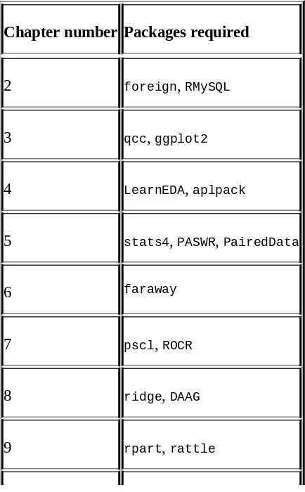
This book uses lot of datasets from the web, statistical text books, and so on. The file format of the datasets have been varied and thus to help the reader, we have put all the datasets used in the book in an R package, RSADBE, which

is the abbreviation of this book’s title. This package will be available from the CRAN website as well as this book’s web page. Thus, whenever you are asked to run data(xyz), the dataset xyz will be available either in the RSADBE

package or datasets package of R.

The book also uses many of the packages available on CRAN. The following table gives the list of packages and the reader is advised to ensure that these packages are installed before you begin reading the chapter. That is, the reader needs to ensure that, as an example,

install.packages(c("qcc”,”ggplot2”)) is run in the R session before

proceeding with Chapter 3, Data Visualization.

Chapter number Packages required

2 foreign, RMySQL

3 qcc, ggplot2

4 LearnEDA, aplpack

5 stats4, PASWR, PairedData

6 faraway

7 pscl, ROCR

8 ridge, DAAG

(57)

(58)

Python installation and setup

The major change in the second edition is augmenting the book with parallel Python programs. The reader might ask the all-important one word question Why? A simple reason, among others, is this: R has an impressive 11,212 packages, and the quantum of impressiveness for Python’s 11,4368 is left to the reader.

Of course, it is true that not all of these Python packages are related to data analytics. The number of packages is as of the date August 11, 2017.

Importantly, the purpose of this book is to help the R user learn Python easily and vice versa. The main source of Python would be its website:

https://www.python.org/:

Version- A famous argument debated among Python users is related to the choice of version 2.7 or 3.4+. Though the 3.0 version has been available since a decade earlier from 2008, the 2.7 version is still too popular and shows no signs of fading away. We will not get into the pros and cons of using the versions and will simply use the 3.4+ version. The author has run the programs in 3.4 version Ubuntu and 3.6 version in Windows and the code ran without any problems. The users of the 2.7 version might be disappointed, though we are sure that they can easily adapt it to their machines. Thus, we are providing the code for the 3.4+ version of Python.

Ubuntu OS already has Python installed and the version that comes along with it is 2.7.13-2. The two lines of code can be run in the gnome-terminal to update Python to the 3.6 version:

sudo apt-get update

sudo apt-get install python3.6

The Windows version can be easily downloaded from

(59)

(60)

Using pip for packages

Additional packages as required need to be installed separetely. pip is the

package manager for Python. If any software is required, we can run the following line as the Python prompt:

pip install package

The table of packages required according to the chapters is given in the following table:

Chapter number Python Packages

2 os, numpy, pandas, pymysql, pickle

3 os, numpy, pandas, matplotlib

4 os, numpy, pandas, matplotlib

5 os, numpy, pandas, matplotlib, scipy

6 os, numpy, pandas, matplotlib, scipy

7 os, numpy, pandas, matplotlib, sklearn pylab, pysal, statsmodels

8 os, numpy, pandas, matplotlib, sklearn, pylab, statsmodels

9 os, numpy, pandas, matplotlib, sklearn

(61)

IDEs for R and Python

The Integrated Development Environment or IDE- most users do not use the software frontend these days. IDEs are convenient for many reasons and the uninitiated reader can search for the keyword. In very simple terms, the IDE may be thought of as the showroom and the core software as the factory. The RStudio appears to be the most popular IDE for R and Jupyter Notebook for Python.

The website for RStudio is https://www.rstudio.com/ and for Jupyter Notebook, it is http://jupyter.org/. The authors of the RStudio version are shown in the following screenshot:

We will not delve into details on the IDEs and the role they play. It is good enough to use them. More details about the importance of IDEs can be easily obtained on the web, and especially Wikipedia. An important Python

(62)

Anaconda-Python predators and how their names fascinate the software programmers. The Anaconda distribution is available at

https://www.continuum.io/downloads and we recommend the reader to use the same. All the Python programs are run on the Jupyter Notebook IDE. The authors of the Anaconda Prompt are shown in the following screenshot:

The code in the jupyter notebook has not yet run. And if you enter that on

your Anaconda Prompt and hit the return key, the IDE will be started. The frontend of the Jupyter notebook, which will be opened in your default

internet browser, looks like the following:

Now, an important question is the need of different IDEs for different software. Of course, it is not necessary. The R software can be integrated with the Anaconda distribution, particularly with options later in the Jupyter IDE. Towards this, we need to run the code conda install -c r

r-essentials in the Anaconda Prompt. Now, if you click on the New

(63)

(64)

(65)

The companion code bundle

After the user downloads the code bundle, RPySADBE.zip, from the

publisher’s website, the first task is to unzip it to a local machine. We encourage the reader to download the code bundle since the R and Python code in the ebook might be in image format and it is a futile exercise to key in long programs all over again.

The folder structure in the unzipped format will consist of two folders: R and Python. Each of these chapters further consists of 10 sub-folders, one folder

for each chapter. R software has a special package for itself as RSADBE

available on CRAN. Thus, it does not have a Data sub-folder with the

exception of Chapter 2, Import/Export Data. The chapter level folders for R will contain two sub-folders: Output and SRC. The SRC folder contains a file

named Chapter_Number.R, which consists of all code used in the package.

The Output folder contains a Microsoft Word document named

Chapter_Number.doc. The reader is given an exercise to set up the Markdown

settings; search for it on the web. The Chapter_Number.doc is the result of

running the R file Chapter_Number.R. The graphics in the Markdown files will

be different from the ones observed in the book.

Python’s chapter sub-folders are of three types: Data, Output, SRC. The

required Comma Separated Values (CSV) data files are available in the

Data folder while the SRC folder consists of the Python code file,

Chapter_Number.py. The output file as a consequence of running the Python

file in the IDE is saved as a Chapter_Number_Title.ipynb file. In many

cases, the graphics generated by either R or Python for the same purpose yields the same display.

Since the R software has been run first and the explanation with the

interpretation given following it, we have given the corresponding Python program, which is different; the graphical output is not necessarily produced in the book. In such cases, the ipynb files would come in handy as they

(66)

Here’s a final word about executing the R and Python files. The author does not have access about the path of the unzipped folder. Thus, the reader needs to specify the path appropriately in the R and Python files. Most likely, the reader would have to replace MyPath by /home/user/RPySADBE or

C:/User/Documents/RPySADBE.

(67)

Discrete distributions

The previous section highlights the different forms of variables. The variables such as Gender, Car_Model, and Minor_Problems possibly take one of the

finite values. These variables are particular cases of the more general class of discrete variables.

It is to be noted that the sample space of a discrete variable need not be finite. As an example, the number of errors on a page may take values on the set of positive integers, {0, 1, 2, …}. Suppose that a discrete random variable X can take values among with respective probabilities

, that is, . Then, we require that the probabilities be non-zero and further that their sum be 1:

where the Greek symbol represents summation over the index i.

The function is called the probability mass function (pmf) of the discrete RV X. We will now consider formal definitions of important families of discrete variables. The engineers may refer to Bury (1999) for a detailed collection of useful statistical distributions in their field. The two most

important parameters of a probability distribution are specified by mean and variance of the RV X.

(68)

The mean is a measure of central tendency, whereas the variance gives a measure of the spread of the RV.

The variables defined so far are more commonly known as categorical variables. Agresti (2002) defines a categorical variable as a measurement scale consisting of a set of categories.

Let us identify the categories for the variables listed in the previous section. The categories for the Gender variable are male and female; whereas the car

category variables derived from Car_Model are hatchback, sedan, station

wagon, and utility vehicles. The Minor_Problems and Major_Problems

variables have common but independent categories, yes and no; and, finally, the Satisfaction_Rating variable has the categories, as seen earlier, Very Poor, Poor, Average, Good, and Very Good. The Car_Model variable is just a

set of labels of the name of car and it is an example of a nominal variable.

Finally, the output of the Satistifaction_Rating variable has an implicit

order in it: Very Poor < Poor < Average < Good < Very Good. It may be

apparent that this difference poses subtle challenges in their analysis. These types of variables are called ordinal variables. We will look at another type of categorical variable that has not popped up thus far.

Practically, it is often the case that the output of a continuous variable is put in a certain bin for ease of conceptualization. A very popular example is the categorization of the income level or age. In the case of income variables, it has become apparent in one of the earlier studies that people are very

conservative about revealing their income in precise numbers.

(69)

(70)

Discrete uniform distribution

A random variable X is said to be a discrete uniform random variable if it can

take any one of the finite M labels with equal probability.

As the discrete uniform random variable X can assume one of the 1, 2, …, M with equal probability, this probability is actually . As the probability remains the same across the labels, the nomenclature uniform is justified. It might appear at the outset that this is not a very useful random variable.

However, the reader is cautioned that this intuition is not correct. As a simple case, this variable arises in many cases where simple random sampling is needed in action. The pmf of a discrete RV is calculated as:

A simple plot of the probability distribution of a discrete uniform RV is demonstrated next:

> title("A Dot Chart for Probability of Discrete Uniform RV”)

Tip

Downloading the example code

(71)

Probability distribution of a discrete uniform random variable

Note

The R programs here are indicative and it is not absolutely necessary that you follow them here. The R programs will actually begin from the next chapter and your flow won’t be affected if you do not understand certain aspects of them.

(72)

(73)

Binomial distribution

Recall the second question in the Experiments with uncertainty in computer science section, which asks: How many machines are likely to break down after a period of 1 year, 2 years, and 3 years?. When the outcomes involve uncertainty, the more appropriate question that we ask is related to the probability of the number of break downs being x.

Consider a fixed time frame, say 2 years. To make the question more generic, we assume that we have n number of machines. Suppose that the probability of a breakdown for a given machine at any given time is p. The goal is to obtain the probability of x machines with the breakdown, and implicitly (n-x) functional machines. Now consider a fixed pattern where the first x units have failed and the remaining are functioning properly. All the n machines function independently of other machines. Thus, the probability of observing x machines in the breakdown state is .

Similarly, each of the remaining (n-x) machines have the probability of (1-p) of being in the functional state, and thus the probability of these occurring together is . Again, by the independence axiom value, the

probability of x machines with a breakdown is then given by . Finally, in the overall setup, the number of possible samples with a

breakdown being x and (n-x) samples being functional is actually the number of possible combinations of choosing x-out-of-n items, which is the

combinatorial .

As each of these samples is equally likely to occur, the probability of exactly

(74)

as:

The pmf of a binomial distribution is sometimes denoted by . Let us now look at some important properties of a binomial RV. The mean and variance of a binomial RV X are respectively calculated as:

Note

As p is always a number between 0 and 1, the variance of a binomial RV is always lesser than its mean.

Example 1.3.1: Suppose n = 10 and p = 0.5. We need to obtain the

probabilities p(x), x=0, 1, 2, …, 10. The probabilities can be obtained using the built-in R function, dbinom. The function dbinom returns the probabilities

of a binomial RV.

The first argument of this function may be a scalar or a vector according to the points at which we wish to know the probability. The second argument of the function needs to know the value of n, the size of the binomial

distribution. The third argument of this function requires the user to specify the probability of success in p. It is natural to forget the syntax of functions and the R help system becomes very handy here. For any function, you can get details of it using ? followed by the function name. Please do not insert a

(75)

> n <- 10; p <- 0.5

> p_x <- round(dbinom(x=0:10, n, p),4) > plot(x=0:10,p_x,xlab=”x”, ylab=”P(X=x)”)

The R function round fixes the accuracy of the argument up to the specified

number of digits.

Binomial probabilities

(76)

utility facets for the binomial distribution. The three facets are p, q, and r.

These three facets respectively help us in computations related to cumulative probabilities, quantiles of the distribution, and simulation of random numbers from the distribution. To use these functions, we simply augment the letters with the distribution name, binom, here, as pbinom, qbinom, and rbinom.

There will be, of course, a critical change in the arguments. In fact, there are many distributions for which the quartet of d, p, q, and r are available; check ?Distributions.

The Python code block is the following:

Example 1.3.2: Assume that the probability of a key failing on an 83-set keyboard (the authors, laptop keyboard has 83 keys) is 0.01. Now, we need to find the probability when at a given time there are 10, 20, and 30

non-functioning keys on this keyboard. Using the dbinom function, these

probabilities are easy to calculate. Try to do this same problem using a

scientific calculator or by writing a simple function in any language that you are comfortable with:

(77)

believe that maybe something is going wrong. As a check, the sum clearly equals 1. Let us have a look at the problem from a different angle. For many x values, the probability p(x) will be approximately zero. We may not be interested in the probability of an exact number of failures though we are interested in the probability of at least x failures occurring, that is, we are interested in the cumulative probabilities . The cumulative probabilities for binomial distribution are obtained in R using the pbinom

function. The main arguments of pbinom include size (for n), prob (for p),

and q (the at least x argument). For the same problem, we now look at the

cumulative probabilities for various p values:

> n <- 83; p <- seq(0.05,0.95,0.05) > x <- seq(0,83,5)

> i <- 1

> plot(x,pbinom(x,n,p[i]),”l”,col=1,xlab=”x”,ylab= + expression(P(X<=x)))

> for(i in 2:length(p)) { points(x,pbinom(x,n,p[i]),”l”,col=i)}

Cumulative binomial probabilities

(78)

(79)

Hypergeometric distribution

A box of N = 200 pieces of 12 GB pen drives arrives at a sales center. The

carton contains M = 20 defective pen drives. A random sample of n units is

drawn from the carton. Let X denote the number of defective pen drives obtained from the sample of n units. The task is to obtain the probability distribution of X. The number of possible ways of obtaining the sample of

size n is . In this problem, we have M defective units and N-M working

pen drives, and x defective units can be sampled in different ways and

n-x good units can be obtained in distinct ways. Thus, the probability distribution of the RV X is calculated as:

where x is an integer between and . The RV

is called the hypergeometric RV and its probability distribution is called the hypergeometric distribution.

Suppose that we draw a sample of n = 10 units. The dhyper function in R

can be used to find the probabilities of the RV X, assuming different values:

(80)

> n = 10 > x = 0:11

> round(dhyper(x,M,N,n),3)

[1] 0.377 0.395 0.176 0.044 0.007 0.001 0.000 0.000 0.000 0.000 0.000 0.000

The equivalent Python implementation is as follows:

(81)

Negative binomial distribution

Consider a variant of the problem described in the previous subsection. The 10 new desktops need to be fitted with an add-on, five megapixel external cameras, to help the students attend a certain online course. Assume that the probability of a non-defective camera unit is p. As an administrator, you keep on placing orders until you receive 10 non-defective cameras. Now, let X denote the number of orders placed for obtaining the 10 good units. We denote the required number of successes by k, which in this discussion has been k = 10. The goal in this unit is to obtain the probability distribution of X.

Suppose that the xth order placed results in the procurement of a kth non-defective unit. This implies that we have received (k-1) non-non-defective units

among the first (x-1) orders placed, which is possible in distinct ways. At the xth order, the instant of having received the kth non-defective unit, we have k successes and x-k failures. Thus, the probability distribution of the RV is calculated as:

(82)

A particular and important special case of the negative binomial RV occurs for k = 1, which is known as the geometric RV. In this case, the pmf is calculated as:

Example 1.3.3. (Baron (2007). Page 77) sequential testing: In a certain setup, the probability of an item being defective is (1-p) = 0.05. To complete the lab setup, 12 non-defective units are required. We need to compute the probability that at least 15 units need to be tested. Here we make use of the cumulative distribution of the negative binomial distribution pnbinom

function available in R. Similar to the pbinom function, the main arguments

that we require here would be size, prob, and q. This problem is solved in a

single line of code:

> 1-pnbinom(3,size=12,0.95) [1] 0.005467259

Note that we have specified 3 as the quantile point (at least x argument) as the

size parameter of this experiment is 12 and we are seeking at least 15 units that translate into three more units than the size of the parameter. The

pnbinom function computes the cumulative distribution function and the

requirement is actually the complement and hence the expression in the code is 1–pnbinom. We may equivalently solve the problem using the dnbinom

(83)

> 1-(dnbinom(3,size=12,0.95)+dnbinom(2,size=12,0.95)+dnbinom(1, + size=12,0.95)+dnbinom(0,size=12,0.95))

(84)

Poisson distribution

The number of accidents on a 1 km stretch of road, the total calls received during a 1-hour slot on your mobile, the number of "likes” received on a status on a social networking site in a day, and similar other cases, are some of the examples that are addressed by the Poisson RV. The probability distribution of a Poisson RV is calculated as:

Here, is the parameter of the Poisson RV with X denoting the number of events. The Poisson distribution is sometimes also referred to as the law of rare events. The mean and variance of the Poisson RV are surprisingly the

same and equal , that is, .

Example 1.3.4: Suppose that Santa commits errors in a software program with a mean of three errors per A4-size page. Santa’s manager wants to know the probability of Santa committing 0, 5, and 20 errors per page. The R

function, dpois, helps to determine the answer:

> dpois(0,lambda=3); dpois(5,lambda=3); dpois(20, lambda=3) [1] 0.04978707

[1] 0.1008188 [1] 7.135379e-11

(85)

Statistical Application Development with R and Python Second Edition pdf pdf

Table of Contents