COMPREHENSIVE COMPARISON OF TWO IMAGE-BASED POINT CLOUDS
FROM AERIAL PHOTOS WITH AIRBORNE LIDAR FOR LARGE-SCALE MAPPING
E. Widyaningrum a, b*, B.G.H Gorte a*
a Dept. of Geoscience and Remote Sensing, Civil Engineering and Geosciences Faculty, Technical University of Delft, Netherlands - (e.widyaningrum, B.G.H.Gorte)@tudelft.nl
b Centre for Topographic Base Mapping and Toponyms, Geospatial Information Agency, Bogor, Indonesia – [email protected]
ISPRS ICWG III/IVb
KEY WORDS: Point Clouds, Aerial Photos, LiDAR, Semi Global Matching, Structure from Motion, Comparison Analyses
ABSTRACT:
The integration of computer vision and photogrammetry to generate three-dimensional (3D) information from images has contributed to a wider use of point clouds, for mapping purposes. Large-scale topographic map production requires 3D data with high precision and accuracy to represent the real conditions of the earth surface. Apart from LiDAR point clouds, the image-based matching is also believed to have the ability to generate reliable and detailed point clouds from multiple-view images. In order to examine and analyze possible fusion of LiDAR and image-based matching for large-scale detailed mapping purposes, point clouds are generated by Semi Global Matching (SGM) and by Structure from Motion (SfM). In order to conduct comprehensive and fair comparison, this study uses aerial photos and LiDAR data that were acquired at the same time. Qualitative and quantitative assessments have been applied to evaluate LiDAR and image-matching point clouds data in terms of visualization, geometric accuracy, and classification result. The comparison results conclude that LiDAR is the best data for large-scale mapping.
* Corresponding author
1. INTRODUCTION
Faithful 3D reconstruction of urban environments represents a topic of great interest in photogrammetry, remote sensing and computer vision expertise, as it provides an important prerequisite for applications such as city modelling, scene interpretation or urban accessibility analysis (Weinmann and Jutzi, 2015). Several remote-sensing techniques and image-based photogrammetric approaches allow an efficient generation of massive 3D point clouds of our physical environment. The efficient processing, analysis, exploration, and visualization of massive 3D point clouds constitute challenging tasks for applications, systems, and workflows in disciplines such as urban planning, environmental monitoring, disaster management, and homeland security (Richter, Behrens and Doellner, 2013). Progressive development in 3D point clouds creates various option to generate 3D point clouds data especially in the image-based matching construction. This attracts the map producer to use these as an alternative to accelerate the base map provision in efficient and effective way, compliant with the map standard. Fully automated image-based creation of dense point clouds with an elevation measurement at each pixel is nowadays feasible at low cost and makes the technology competitive with LiDAR-based surface measurements (Leberl et al., 2010).
One of the advantages of image-based matching is its ability to encode the points with spectral RGB (Red, Green, and Blue) information, which is potentially useful to obtain a better classification. On the other hand, LiDAR data acquired from the Airborne Laser Scanning (ALS) system has many benefits with
its capability to penetrate the dense canopies and produce fusion or integration. As stated by Mishra and Zhang, (2012), a complete surface representation that is presenting both spectral and 3D coordinate information is important for many remote sensing applications, such as classification, feature extraction, building construction, canopy modelling, 3D city modelling etc. Much research has been done in photogrammetry, remote sensing and computer vision to find and further exploit the best fit of photogrammetric and LiDAR data integration.
An accurate registration of LiDAR and optical image dataset remains an open problem due to their different characteristics (Mishra and Zhang, 2012). Fusion of optical images and LiDAR point clouds has been proposed, but the current state is still not satisfying in some applications (Zhang and Lin, 2016). The investigation into the use of aerial images and LiDAR data to detect building changes is carried on but has limitation to extract building boundaries due to the noise and uncertainties of photogrammetric point clouds (Du et al., 2016). Chiabrando et al. (2015) investigate the orthophoto generation from SfM and conclude that traditional digital photogrammetric technique was the best solution for a complete and accurate 3D survey. Therefore, it is necessary to examine point cloud characteristics in order to assess data quality and assure suitability for different 3D applications.
This study investigates the characteristics of different point clouds and identifies the advantages and limitations to help The International Archives of the Photogrammetry, Remote Sensing and Spatial Information Sciences, Volume XLII-2/W7, 2017
readers selecting suitable methods for further 3D application, especially for large-scale mapping. By using different point clouds that have no time gap, this study is expected to resume a comprehensive, fair, and reliable comparison based on qualitative and quantitative analysis.
2. STUDY AREA AND DATA DESCRIPTION
2.1 Study Area
The study area is located in Mataram City of Lombok Island of Indonesia. This area has urban-coastal characteristics and low-flat topography. It covered an area about 430 meters by 1320 meters or 56 ha.
Figure 1. The study area, LiDAR data coverage, and the footprint of aerial photo frames
2.2 Data Description
The primary data in this study consist of aerial photos and a LiDAR point cloud. Both datasets were acquired by the same aircraft platform at the same time, on June 17, 2016. The datasets use WGS1984 as horizontal reference and EGM2008 as the vertical datum. Further details of the datasets are described below:
a. Aerial Photo
Digital medium format aerial photos were taken by a Leica RCD30 instrument with a focal length of 53 mm and combined with Exterior Parameters (EO) and pre-marking Ground Control Points (GCP) datasets. The RGB images size is 6732 x 9000 pixels and has 15 cm ground sampling distance. The aerial photos were acquired with a minimum overlap of 60% and sidelap of 40%. Based on the independent check points measured by dual-frequency geodetic GPS, the horizontal geometric accuracy (CE90) of aerial photo is 0.406 meter and the vertical accuracy (LE90) is 0.390 meter.
b. LiDAR
The total number of LiDAR point clouds in the study area is 6.392.505 points, acquired from Leica ALS70 instrument. The LiDAR point cloud has a density of 11 points per meters (ppm). The vertical accuracy of LiDAR point clouds data which measured from 70 ground check points by using dual-frequencies geodetic GPS is 0.198 meter.
3. GENERATION OF IMAGE-BASED MATCHING POINTS
3.1 Image-based Matching Points using SfM Approach
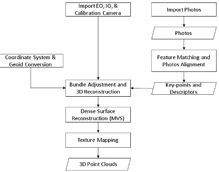
The process of estimating the 3D geometry (structure) and camera pose (motion) is commonly known as Structure from Motion (SfM). This algorithm can reconstruct a sparse 3D point cloud of large complex scenes from series of overlapping photos (Snavely et al., 2006). The SfM approach computes simultaneously both this relative projection geometry and a set of sparse 3D points. To do this, it extracts corresponding image features from a series of overlapping photographs captured by a camera moving around the scene (Verhoeven et al., 2013). SfM relies on algorithms that detect and describe local features for each image and then match those two-dimensional (2D) points throughout the multiple images. Using this set of matched points as input, SfM computes the position of those interest points in a local coordinate frame (also called model space) and produces a sparse 3D point clouds that represent the geometry or structure of the scene. As mentioned previously, the camera pose and internal camera parameters are retrieved also (Szeliski, 2011). Afterward, some details are given about the subsequent process, the multi-view stereo (MVS) is applied as the last stage by using the SfM result as an input to generate a dense 3D model (Verhoeven, 2013).
Figure 2. The SfM-based point clouds generation workflow
In this study, the SfM-based 3D point cloud generation uses the Agisoft Photoscan software. Once the pertinent photos are imported into chunks, the feature matching and photo alignment is started. At this stage, tie points are detected based on stable viewpoint and lighting variations and generates the descriptor based on its local neighbourhood. The descriptors are then used to aligning the overlapping photos. This algorithm is similar to the well-known SIFT (Scale-Invariant Feature Transform) algorithm (Agisoft Forum, 2011) in resulting a sparse point cloud. The next step is find the initial camera location and refine them by using bundle adjustment algorithm based on photos Interior Parameter (IO) and Exterior Parameter (EO). Finally, the dense image matching points are constructed based on multi view algorithm, as one of the used approach. The last step is texture mapping to perform a texture and assigning the RGB information.
In this matching point generation process, there are two necessary conversions during the image-base matching process The International Archives of the Photogrammetry, Remote Sensing and Spatial Information Sciences, Volume XLII-2/W7, 2017
because of the digital-frame airborne aerial photos data has its own calculated EO and IO. The first conversion is the EO parameter conversion, from omega phi kappa to roll pitch yaw. The second conversion is datum reference transformation from elipsoid to geoid since the Photoscan set the vertical reference in ellipsoid automatically.
The SfM-based point cloud is improved by using Iterative Closest Points (ICP) algorithm to get a better alignment. ICP is conducted to minimize the position difference between two point clouds by estimating the transformation parameters iteratively with the assumption of the existence of a good a priori alignment (Gressin, Mallet, David, 2012).
The SfM-based point clouds result has average point density 25,01 points per meter square and produce 14.780.288 points in total within the study area.
3.2 Image-based Matching Points using SGM Approach
The Semi Global Matching (SGM) stereo method is based on the idea of pixel-wise matching cost (disparity) of Mutual Information (MI) for compensating the radiometric differences of input images and uses a smoothness constraint. Accurate and fast pixel-wise matching is done by optimizing the pathwise of a global cost function (Hirschmueller, 2008). The core algorithm of SGM aggregates the matching costs under consideration of smoothness constraints. The minimum aggregated cost leads to the disparity map for a stereo pair and subsequently to textured 3D point clouds in object space (Nebiker et al., 2012).
The large numbers of matches found in this way allow for the creation of very detailed 3D models. The SGM algorithm maintains sharper object boundaries than local methods and implements mutual information (MI) based matching instead of intensity based matching because it “is robust against many complex intensity transformations and even reflections” (Hirschmueller, 2005).
The SGM-based matching points generation in this study is carried out by using XPro SGM of Erdas Imagine Photogrammetry. The threshold for disparity difference assigned in the process is 1 with the pyramid levels 0. The disparity threshold is the maximum blunder allowed when doing reverse matching. Thus, this study allowed the disparity difference for one pixel in maximum. The higher the disparities value, the more points will be generated but this may also increases noises. On the other hand, disparity threshold 0 means no difference is allowed and it will be harder to find the matched points. The pyramid is built to speed up the run time processing and faster display, thus this study uses the photos original resolution for the statistics calculation. Imagine Photogrammetry uses binomial interpolation (Kernel) algorithm.
Figure 3. The SGM-based point clouds generation workflow
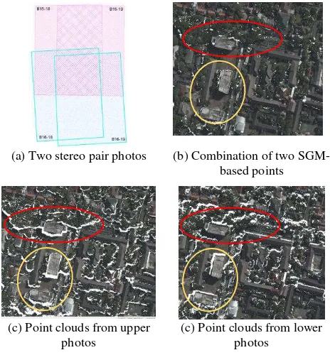
The generated SGM-based point clouds result has an average point density 25,25 points per meter square. The total number of extracted 3D points in the study area is 14.923.383 points. The XPro SGM producing point clouds in each overlap areas of two photos and this study uses minimum overlap 50%. Thus, there are two point clouds file generated in this step that generated from the overlap of two photos in flight line 15 (or upper part photos) and flight line 16 (lower part photos). There are overlap points in both dataset and there are certain conditions where both point clouds dataset able to complement each other in filling voids or holes caused by shadows of high objects as shown in Figure 4.
(a) Two stereo pair photos (b) Combination of two SGM-based points
(c) Point clouds from upper photos
(c) Point clouds from lower photos
Figure 4. The SGM point clouds result
3.3 DEM Generation from Point Clouds
Each of the image-based point clouds as well as the LiDAR point cloud is resampled into a raster DEM and then used as the basis of visual comparison and quantitative evaluation. The DEMs in this study are triangulated from each point clouds by using same parameter values and have 0,25 meter pixel size. The International Archives of the Photogrammetry, Remote Sensing and Spatial Information Sciences, Volume XLII-2/W7, 2017
Figure 5. The DEM of SGM-based surface representation
The hill-shaded DEM helps to visualized the surface, especially in detecting the possible noise in flat surfaces. Figure 5 shows that the integration of two SGM-based point cloud creates more noise especially in the planar surface.
4. RESULT AND DISCUSSION
This study uses qualitative and quantitative analysis to evaluate and compare the point cloud datasets. The qualitative analysis uses criteria such as the completeness, shape, sharpness, and flat-planes based on data visualization, while the quantitative approach uses geometric and classification accuracy criteria. The comparison of point clouds in this study uses LiDAR point cloud data as the reference.
LiDAR SfM-based SGM-based Total Points 6.392.505 14.780.288 14.923.383
Point Density 11 25.01 25.25 Table 1. Resume of the comparable point clouds
4.1 Visualization
Visualization is the easiest way to do general comparison and preliminary evaluation as well as to identify the problems. Moreover, some application still need human perspective point of view and visual interpretation in certain level or process phase, especially during quality control step. Thus, this study employs some criteria to make comparison of point clouds datasets based on their visualization.
The image-base matching has a superior ability over LiDAR point cloud in providing a RGB information. Both image-based matching methods are able to generate RGB point clouds with exact colours as aerial photos, as shown in Figure 7A.
(a) LiDAR
(b) SfM-based point cloud
(c) SGM-based point cloud
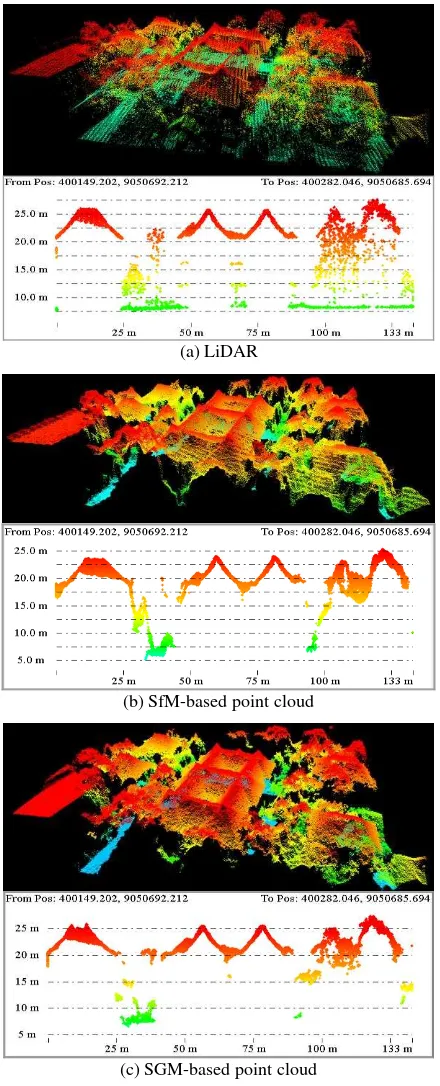
Figure 6. The 3D visualization and profile of point clouds
4.1.1 The 3D Profiles: A 3D profile and visualization of different point clouds shows definite differences in terms of point density, details, and noise. The 3D profile shows that LiDAR system is able to detect small and low vegetation and also the middle part of high trees. This may necessary for some applications but may also become disadvantages for some other applications, especially for trees or canopies modelling. Ground points are better constructed in LiDAR than in image-based matching data due to LiDAR ability penetrates dense vegetation. The International Archives of the Photogrammetry, Remote Sensing and Spatial Information Sciences, Volume XLII-2/W7, 2017
The SfM-based has similar point density as SGM-based data, but the 3D profile shows that SfM-based yields more noise on a planar roof than SGM-based as shown in Figure 6.
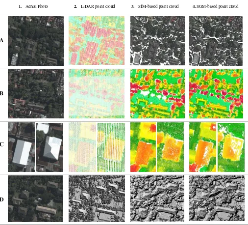
4.1.2 Completeness and Voids: In the study area, almost all of objects in the surface are constructed and presented in each of point clouds data except for some dense trees. Many voids or holes exist in the image-based matching point clouds due to dark shadow in the image or insufficient texture of object surfaces. The most significant different found in this study area is the absence of some dense trees in the SfM-based point clouds as shown in Figure 7B. The problems in constructing points of a high dense trees may failed due to positional changes in the corresponding images, because tree leafs are moved by the wind, which then also creates different spectral value and resulting zero key points during the SfM processing.
In the study area, there are some small voids found on zinc-metal building roof surface (Figure 7C) and SGM-based is likely producing more small voids on zinc-metal roofs than in SfM-based data. Metal surface has low texture and susceptible to sun angle. Different acquisition angles cause different reflectance value of metal surface in photos, which then leads to harder matching process.
Moreover, there is an absence of points on very high buildings and the surroundings, such as towers.
4.1.3 Flatness and Sharpness of Built Objects: The hill-shaded DEMs generated from point cloud show LiDAR has better visualization in performing building roof edges. As seen in Figure 7D., the building roofs are looks smoother in LiDAR DEM than in image-based matching DEM data.
1. Aerial Photo 2. LiDAR point cloud 3. SfM-based point cloud 4.SGM-based point cloud
A
B
C
D
Figure 7. Visual comparison of aerial photos, LiDAR, SfM-based, and SGM-based data point clouds The International Archives of the Photogrammetry, Remote Sensing and Spatial Information Sciences, Volume XLII-2/W7, 2017
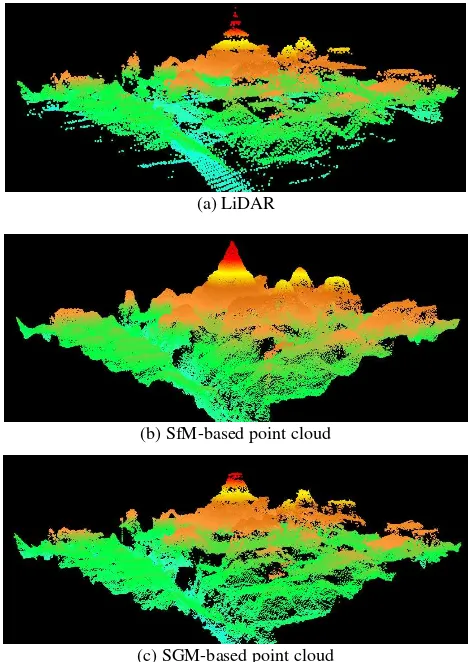
4.1.1 Peak Representations: The 3D visualization of point clouds as shown in Figure 8. is shows that the SfM-based points are able to detect a small peaks in the roof but have more noise in detecting the objects surface. On the other hand, the SGM-based point cloud is not able to detect the small peak but it has less noise so that it has sharper edges and shapes especially in detecting the building roof surface. The LiDAR points are still the best for detecting the small high objects as well as the object details.
(a) LiDAR
(b) SfM-based point cloud
(c) SGM-based point cloud
Figure 8. 3D point cloud visualization of small sharp peak object
4.2 Geometric Accuracy
Evaluation of the geometric accuracy is carried out to define the relative position of each point cloud in comparison with LiDAR data in X, Y and Z position. The check points are assigned based on visibility and the sharpness of the object in the generated DEMs. The check points should also well-distributed and well-identified in all of DEM. There are 42 check points calculated and used within the study area.
(a) Check point distribution
(b) LiDAR check points
(c) SfM Check points
(d) SGM Check points
Figure 9. Check-points placement for geometric accuracy assessment
The geometric accuracy is calculated by adopting the US-NMAS (United States National Map Accuracy Standards) formula as follows:
Horizontal accuracy (CE90) = 1,5175 x RMSEr Vertical accuracy (LE90) = 1,6499 x RMSEz
Where:
RMSEr = Root Mean Square Error in x and y position RMSEz = Root Mean Square Error in z position
The RMSE value is calculated from the X, Y, and Z position of each appointed check points on SfM, SGM, and LiDAR data. The result of relative vertical accuracy of SfM data achieves 0.81 meters while the SGM is 0.62 meters. For the horizontal accuracy, the SfM data achieves 1.79 meters and the SGM is 0.47 meters.
4.3 Vertical Distance Differences
The M3C2 technique allows rapid analysis of large point clouds with complex surfaces that span a range of surface orientations (Barnhart & Crosby, 2013).
Lague et al. (2012) invented an accurate 3D comparison of complex topography. Once the normal is defined for the core point i, it is used to project i onto other cloud at scale D (called projection scale). This scale use to define the average positions i1 and i2 of each subset of points in the neighbourhood of i. This is done by defining a cylinder radius (d/2) whose axis goes through i and oriented along the normal vector N. The cylinder intercept two subsets of points of size S1 and S2. Projecting each of subsets on the axis of a cylinder gives two distributions of distances (with an origin i). The mean of the distribution gives the average position of the points subset along the normal The International Archives of the Photogrammetry, Remote Sensing and Spatial Information Sciences, Volume XLII-2/W7, 2017
direction, i1 and i2, and two standard deviations give local estimation of the point cloud roughness σ1(d)and σ2(d) along the normal direction. If outliers are expected in the data (such as vegetation), i1 and i2 can be defined as the median of the distance distribution and the roughness is measured by the interquartile range. The local distance between the two clouds L is given by the distance between i1and i2.
Figure 10. Illustration of M3C2 concept
Averaging point cloud position is done by defining the core points within the cylinder. The core points are used to define points for the cylinder and it is where the distance calculation is started. It is necessary to define the minimum sampling distance and scale, since the approximate distance (L) between two point clouds is computed once core point is selected and find the nearest points in the cylinder. This study uses normal orientation in Z direction to measure the surface height differences.
(a) SfM to LiDAR (b) SGM to LiDAR
Figure 11. The M3C2 vertical distance of two point clouds
The M3C2 distance provides the vertical difference range from negative to positive direction of image-based matching point to LiDAR point position. The negative direction means that height value in LiDAR is lower than in image-based matching point cloud, while the positive direction means that height value of LiDAR is higher than image-based matching. The M3C2 distance, as shown Figure 11., is dominated by green colours which means that most of the vertical difference between two point clouds is near to zero.
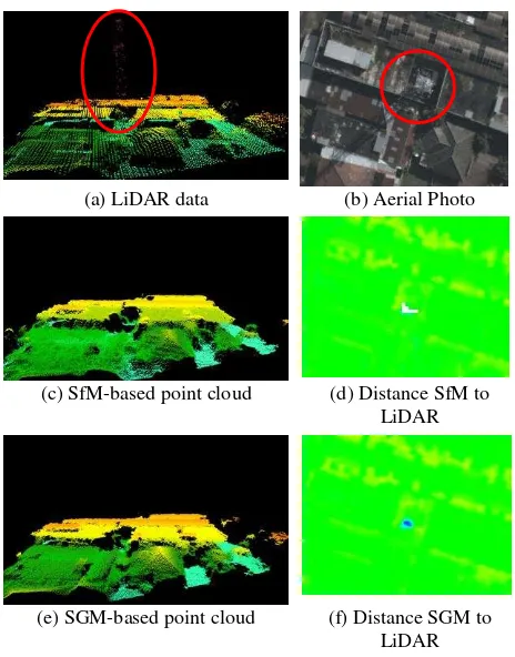
The highest vertical difference between SGM-based to LiDAR in negative direction is detected in the tower and surrounding area. LiDAR data able to construct tower point which has summit height of 48 meters while SGM is only able to detect tower points with 10 meters height. On the other hand, there is a void or hole exist in SfM-based distance since SfM failed to
construct any point of the tower object and its surrounding area. Because a pointed tower is very high, it may looks leaning differently in some corresponding images due to object relief displacement. The image-based matching algorithm may unable to find corresponding pixel of a very high tower metal-made, which have significant differences in position, shape and colour.
(a) LiDAR data (b) Aerial Photo
(c) SfM-based point cloud (d) Distance SfM to LiDAR
(e) SGM-based point cloud (f) Distance SGM to LiDAR
Figure 12. The communication tower in LiDAR and the M3C2 distance to image-based matching point
The highest vertical distance of SGM in positive direction is found in the ground shadow areas of high buildings. In these areas, LiDAR point has lower elevation and it detects the ground accurately. In the same area, SfM is not able to produce the points.
Mostly, a high difference in positive and negative direction for both image-based matching points happens in the shadow area under or near to the high dense trees. The high negative direction difference occurs because LiDAR points have lower elevation than image-based matching points due to LiDAR capabilities in penetrating to ground surface through dense canopies. Furthermore, the high differences in positive direction is mostly caused by insufficient texture information in black shadow areas, or higher disparities level that cause low confident level in image-based matching points.
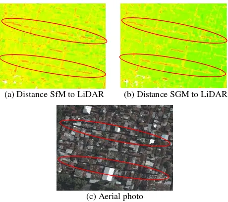
Another distance difference is found along the narrow dark shadowed street areas that are located between dense buildings. The higher M3C2 distance between LiDAR and image-based points is presented in yellow colour in Figure 13. This situation emphasizes that image-based matching has dependency on spectral and object texture to find corresponding pixels. The International Archives of the Photogrammetry, Remote Sensing and Spatial Information Sciences, Volume XLII-2/W7, 2017
(a) Distance SfM to LiDAR (b) Distance SGM to LiDAR
(c) Aerial photo
Figure 13. The distance in narrow shadowed street
4.4 Building Classification Accuracy
Buildings belong to the most important objects to be presented in in maps. Thus, this study also examines the classification correctness of full resolution point clouds in order to have a broader comparison. For the classification accuracy assessment, the samples of polygon building roof are randomly chosen and delineated by manual/visual interpretation. Then, a building classification is carried out for all the point clouds datasets by applying the same planarity methods, parameters, and threshold (minimum height 30 cm, minimum building size 25 square meters and Z tolerance 40 cm). By selecting all of points located inside the polygons, the number of building points that correctly assigned as building and non-building is known. The result shows that all these point clouds has the same correctness percentage for building roof classification.
The classification assessment result shows that point density is not affecting very much the accuracy of point clouds classification.
5. CONCLUSION AND RECOMMENDATION
This study investigates the comparison of different point clouds. There are no time gaps between all the datasets. Understanding the characteristics of LiDAR and image-based matching point clouds should help many applications to select suitable methods, which meet their criteria and specification. We conclude that topographic base mapping production should preferably use LiDAR point cloud data because LiDAR has the capability to penetrate dense vegetation and produce ground points accurately. Image-based matching point clouds are considered an applicable, fast, and low-cost method for any application that
does not require an absolute accuracy of terrain or ground surface, but instead use relative computation. For other applications such as mining, tree, forest, or other surface volumetric calculation, a priori knowledge of the project areas and its surrounding condition (vegetation type and density, urban type, etc) is necessary. Classification accuracy is not improved by using higher point density unless it augmented by RGB information. The building classification result proves that the image-based matching is able to produce stable planar points on the surface with tolerable noise.
In terms of geometric position, significant differences exist between different methods. These geometric differences become a major obstacle for data fusion. Therefore, the objective to integrate the 3D positions of LiDAR and RGB value of image-based matching point clouds accurately for large-scale mapping still needs to be studied further.
ACKNOWLEDGEMENTS
The authors appreciate the Indonesian Geospatial Information Agency (www.big.go.id) for providing the data and PT. Leica Geosystems Indonesia for the Erdas Imagine software support.
REFERENCES
Barnhart, T. B., Crobsy, B. T., 2013. Comparing Two Methods of Surface Change Detection on an Evolving Thermokarst using High-Temporal-Frequency Terrestrial Laser Scanning, Selawik River, Alaska. Remote Sensing, ISSN 2072-4292.
Chiabrando, F., Donadio, E., Rinaudo, F., 2015. SfM for Orthophoto Generation: A Winning Approach for Cultural Heritage Knowledge. International Archives of the
Photogrammetry, Remote Sensing and Spatial Sciences, Vol.
XL-5/W7. 25th International CIPA Symposium, Taipei, Taiwan. Du, S., Zhang, Y., Qin, R., Yang, Z., Zou, Z., Tang, Y., Fan, C., 2016. Building Change Detection using Old Aerial Images and New LiDAR Data. Remote Sensing, ISSN 2072-4292, Vol. 8, Issue 12.
Gressin, A., Mallet, C., David, N., 2012. Improving 3D LiDAR Point Cloud Registration using optimal Neghborhood Knowledge. ISPRS Annals of the Photogrammetry, remote
Sensing and Spatial Information Sciences, XXII ISPRS
Congress, Vol. I-3, Melbourne, Australia.
Hirschmueller, H., 2005. Accurate and Efficient Stereo Processing by Semi-Global Matching and Mutual Information.
IEEE Conference on Computer Vision and Pattern Recognition,
Vol. 2, pp. 807-814, San Diego, USA.
Hirschmueller, H., 2008. Stereo Processing by Semiglobal
Matching and Mutual Information. IEEE Transactions on
Pattern Analysis and Machine Intelligence, Vol. 30, No. 2.
Hirschmueller, H., 2011. Semi-Global Matching – Motivation, Developments and Applications, Stuttgart, Germany
http://www.ifp.uni-stuttgart.de/publications/phowo11/180Hirschmueller.pdf (2 March 2017).
Lague, D., Brodu, N., Leroux, J., 2013. Accurate 3D Comparison of Complex Topography with Terrestrial Laser Scanner: Application to the Rangitikei Canyon (N-Z). ISPRS
Journal Photogrammetry, 10.1016.
Leberl F., Irschara A., Pock T., Meixner P., Gruber M., Scholz S., and Wiechert, A., 2010. Point Clouds: Lidar versus 3D Vision. Photogrammetric Engineering and Remote Sensing, 76 (10): 1123-1134.
Maltezos, E., Kyrkou, A., Ioannidis, C., 2016. LiDAR vs Dense Image Matching Point Clouds in Complex Urban Scenes.
Proceedings SPIE 9688, Fourth International Conference on
Remote Sensing and Geoinformation of the Environment (RSCy2016).
Meyer, M., Bartelsen, J., Hirschmueller, H., Kuhn, A., 2011. Dense 3D Reconstruction from Wide Baseline Image Stets. Outdoor and Large-Scale real-World Scene Analysis. 15th International Workshop on Theoretical Foundations of Computer Vision, Dagstuhl Castle, Germany.
Mishra, R. K., Zhang, Y., 2012. A review of Optical Imagery and Airborne LiDAR Data Registration Methods. The Open
Remote Sensing Journal, 5, 54-63.
Nebiker, S., Cavegn, S., Eugster, H., Laemmer, K., Markram, J., and Wagner, R., 2012. Fusion of Airborne and Terrestrial Image-Based 3D Modelling in Road Infrastructure Management – Vision and First Experiments. International Archives of the
Photogrammetry, Remote Sensing and Spatial Sciences, Vol.
XXXIX-B4, XXII ISPRS Congress, Melbourne, Australia.
Richter, R., Behrens, M., and Doellner J., 2013. Object Class Segmentation of Massive 3D Point Clouds 0f Urban Areas using Point Cloud Topology. International Journal of Remote
Sensing, Vol. 34, Issue 23.
Semyonov, D., 2011. Algorithms used in Photoscan. http://www.agisoft.com/forum/index.php?topic=89.0 (1 March 2017).
Szeliski, R., 2011. Computer Vision: Algorithms and
Applications. Springer.
USGS, 1947. United States National Map Accuracy Standards. Retrieved on April 6th, 2017 from https://nationalmap.gov/standards/pdf/NMAS647.PDF
Verhoeven G., Sevara C., Karel W., Ressl C., Doneus M. and Briese C., 2013. Undistorting the past: New Techniques for Orthorectification of Archaeological Aerial Frame Imagery. In:
Good Practice in Archaeological Diagnostics, pp 31-67.
Weinmann, M., Jutzi, B., 2015. Geometric Point Quality Assessment for the Automated, Markerless, and Robust Registration of Unordered TLS Point Clouds. ISPRS Annals of the Photogrammetry, remote Sensing and Spatial Information
Sciences, XXII ISPRS Congress, Vol. II-5, La Grande Motte,
France.
Zhang, J., Lin, X., 2016. LiDAR Point Cloud Applied to Photogrammetry and Remote Sensing. International Journal of
Image and Data Fusion.