FACULTY OF SCIENCE
Jelena Lueti´c
Measurement of the cross section for
associated production of a W boson and
two b quarks with the CMS detector at the
Large Hadron Collider
DOCTORAL THESIS
FACULTY OF SCIENCE
Jelena Lueti´c
Measurement of the cross section for
associated production of a W boson and
two b quarks with the CMS detector at the
Large Hadron Collider
DOCTORAL THESIS
Supervisor:
Professor Vuko Brigljevi´c, PhD
PRIRODOSLOVNO MATEMATI ˇCKI FAKULTET
Jelena Lueti´c
Mjerenje udarnog presjeka zajedniˇcke
tvorbe W bozona i para b kvarkova
detektorom CMS na Velikom hadronskom
sudarivaˇcu
DOKTORSKI RAD
Mentor:
Prof. dr. sc. Vuko Brigljevi´c
Doktorski rad izra ¯den je na Sveuˇcilištu u Zagrebu, Prirodoslovno-matematiˇckom fakultetu
Mentor: prof. dr. sc. Vuko Brigljevi´c
Doktorski rad ima: 130 stranica
“Each time new experiments are observed to agree with the predictions, the theory survives and our confidence in it is increased; but if ever a new observation is found to disagree, we have to abandon or modify the theory.
At least that is what it is supposed to happen, but you can always question the competence of the person who carried out the observation.”
Abstract
The goal of this thesis is a measurement of the cross section of the pp !W +bb+
X process using the data collected during 2012 at ps = 8 TeV. The data is provided by the Large Hadron Collider (LHC) accelerator at CERN, Geneva and collected by the Compact Muon Solenoid (CMS). The production of a W boson in association with a pair of b quarks (Wbb) in proton collisions has been the topic of many theoretical calculations and simulations. It is however still not well described due to divergences which arise in theoretical calculations, in cases where b quarks are collinear or there is a low energy massless particle irradiated. A precise measurement of Wbb production will allow to further constrain theoretical predictions in the framework of perturbative quantum chromodynamics (pQCD). On the other hand, Wbb is a background in the measurements of di↵erent standard model processes as well as in several searches for physics beyond standard model.
The presence of a W boson is identified through the detection of an energetic, isolated lepton (muon or electron) and a significant amount of missing energy, which indicates the presence of a neutrino. Jets in the detector are identified as collimated sprays of particles. Selected jets are required to be tagged as jets originating from b quarks.
The cross section measurement was performed in the fiducial region defined by a presence of a lepton and exactly two 2 b-tagged jets. The result is quoted separately in the muon and electron channel. The measured values in the two channels are compatible, as predicted by the standard model. The theoretical cross section was derived using MCFM. The measured values are around one standard deviation higher than the predicted theoretical values. The uncertainty on the measured values is dominated by the systematic e↵ects. The largest uncertainties are associated with the b tagging procedure, jet energy scale and jet energy resolution. Reducing these uncertainties in the future, would allow for more sensitive test of perturbative QCD calculation at next-to-leading order.
Acknowledgements
I would like to thank all the people who helped make this thesis see the light of day. Thanks to the colegues from University of Wisconsin-Madison, University of Trieste and CERN, specially to Tom , Andrea and others for all their e↵ort and help during past year. Big thanks to Michele for his guidance, patience and precious comments.
I would like to thank to all the CMS group from Ruder Boˇskovi´c Institute. Thanks to Lucija for being a good friend and listener when I needed one. Thanks to Tanja for all her help and hard work and fruitful discussions, without you this would be nearly half as fun. Thanks to Sre´cko, Senka, Darko, Saˇsa and Benjamin for all the help and interesting discussions over the past few years. Special thanks to my supervisor Vuko Brigljevi´c for helping me and believing in me over the past few years.
Thanks to the Pixel group, specially to Danek, Viktor, Gino, Janos, Urs, Annapaola and others for giving me a chance to work on something new and exciting.
Special thanks to my family for all their support and patience. Without you none of this would be possible.
Goran, thank you for being there for me and making me happy.
Contents
Abstract iii
Acknowledgements iv
Contents v
List of Figures ix
List of Tables xiii
Abbreviations xv
1 Introduction 1
2 Theoretical overview and previous measurements 5
2.1 Standard model overview . . . 6
2.1.1 The bottom quark . . . 8
2.1.2 W boson . . . 9
2.2 W + b jets at hadron colliders . . . 10
2.2.1 Cross sections at hadron colliders . . . 11
2.2.2 Theoretical contributions to Wbb cross section . . . 17
2.2.2.1 Double parton scattering. . . 21
2.3 The previous measurements . . . 25
3 The Large hadron collider 29 3.1 Physics goals for the LHC . . . 30
3.2 Design of the LHC . . . 31
3.3 LHC performance . . . 33
4 The Compact muon solenoid 37 4.1 CMS coordinate system . . . 38
4.2 Solenoid magnet. . . 39 v
Contents
4.3 Inner tracker system . . . 40
4.3.1 Pixel Detector . . . 40
4.3.2 Strip detector . . . 42
4.4 The electromagnetic calorimeter . . . 43
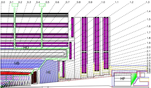
4.5 The hadronic calorimeter . . . 45
4.6 The muon chambers . . . 46
4.7 The trigger . . . 46
4.8 Luminosity measurement . . . 49
5 Physics objects definitions 51 5.1 Electrons. . . 52 5.2 Muons . . . 53 5.3 Lepton isolation . . . 55 5.4 Jets . . . 56 5.4.1 Jet algorithms . . . 56 5.4.2 Jet corrections . . . 59 5.4.3 Jet identification . . . 61
5.4.4 Jets from b quarks . . . 62
5.5 Missing transverse energy . . . 65
6 Event selection and background estimation 67 6.1 Data and Monte Carlo samples . . . 68
6.2 Monte-Carlo corrections . . . 70
6.2.1 Pileup . . . 70
6.2.2 Lepton efficiency measurement . . . 71
6.2.3 b-tagging scale factors . . . 72
6.3 Event selection . . . 75
6.4 Background estimation . . . 76
6.4.1 Top quark background . . . 76
6.4.2 Z+jets . . . 81
6.4.3 W+light jets and W+charm . . . 81
6.4.4 QCD multijets . . . 81
6.4.5 Other backgrounds . . . 83
7 Cross section measurement 87 7.1 Signal extraction method . . . 87
7.2 Systematic uncertainties . . . 90
7.3 Acceptance and efficiency . . . 94
7.4 Results . . . 95
7.4.1 E↵ects of the systematic uncertainties. . . 96
7.4.2 Tests of the fit stability. . . 99
7.4.3 Cross section measurement . . . 100 vi
Contents
7.4.4 Theoretical predictions and comparison with the measurement . . . 101
8 Conclusions 103 9 Strukturirani saˇzetak - Mjerenje udarnog presjeka zajedniˇcke produkcije W bozona i para b kvarkova 105 9.1 Uvod . . . 105
9.2 Teorijski uvod i prethodna mjerenja . . . 106
9.3 LHC . . . 107
9.4 CMS detektor . . . 108
9.5 Rekonstrukcija fizikalnih objekata . . . 109
9.6 Selekcija dogadaja i navaˇznije pozadine . . . 111
9.7 Rezultati . . . 113
9.8 Zakljuˇcak . . . 116
A Lorentz angle measurement in Pixel detector 117 A.1 Grazing angle method . . . 117
A.2 Minimum cluster size method (V-method) . . . 121
Bibliography 123
List of Figures
2.1 List of Standard model elementary particles . . . 7
2.2 A drawing of a proton-proton collision with its decay products. . . 12
2.3 Strong force coupling constant . . . 13
2.4 Drawing of a proton-proton collision . . . 13
2.5 Parton distribution functions for di↵erent momentum transfers . . . 15
2.6 Proton-proton cross sections . . . 16
2.7 LO Wbb Feynmann diagram . . . 18
2.8 Wbb production within 5 flavor scheme . . . 19
2.9 Scale dependence of Wbb cross section . . . 19
2.10 Wbb NLO scale dependence . . . 20
2.11 Double parton scattering . . . 21
2.12 Results of ef f measurements . . . 24
2.13 Atlas Wbb total cross section measurement. . . 26
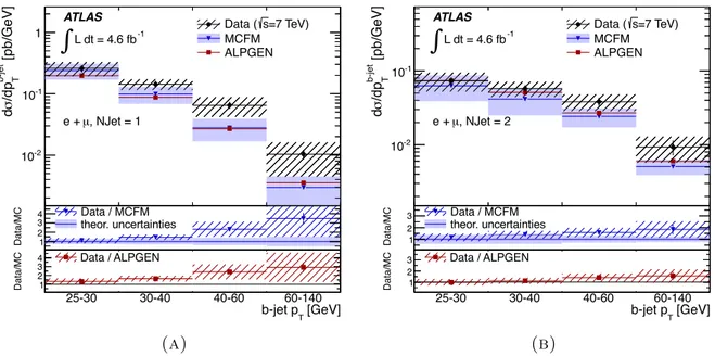
2.14 Measured di↵erential W+b-jets cross-sections as a function of leading b-jet pT . . . 27
2.15 CMS Wbb total cross section measurement . . . 27
3.1 Schematics of Large Hadron Collider . . . 30
3.2 Schematics of dipole magnets . . . 33
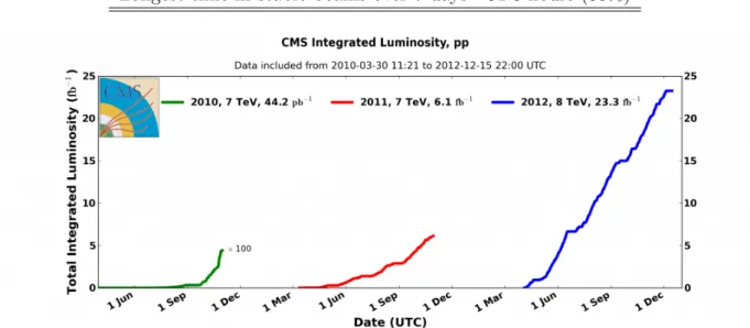
3.3 Luminosity delivered to the CMS experiment. . . 35
4.1 CMS detector . . . 38
4.2 CMS Pixel Detector . . . 41
4.3 CMS Pixel Detector psudorapidity range coverage and efficiency . . . 41
4.4 CMS Strip Detector. . . 43
4.5 CMS Electromagnetic Calorimeter. . . 44
4.6 CMS Hadronic Calorimeter . . . 45
4.7 CMS Muon Chambers . . . 47
4.8 Muon resolution measurements for tracker, muon chambers and combined . 47 4.9 A drawing of CMS Trigger System. . . 48
5.1 An example of configuration of IRC unsafe jet algorithm. . . 57
5.2 Clustering particles into jets with di↵erent algorithms. . . 59
List of Figures
5.3 Total jet energy correction as a function of pseudorapidity of two di↵erent
jet pT values. . . 61
5.4 Total jet energy correction as a function of transverse momentum for four di↵erent⌘ values. . . 62
5.5 Total jet uncertainty and contribution from di↵erent sources in jet pT and ⌘ [54] . . . 63
5.6 Combined secondary vertex discriminator for multijet QCD sample (left) and tt enriched sample(right)[57] . . . 64
5.7 Combined secondary vertex misidentification probability for data and MC for medium working point.[57] . . . 65
6.1 Number of primary vertices before and after the pileup reweighing procedure. 71 6.2 Muon identification and isolation efficiencies usingtag and probe method. . 73
6.3 Muon trigger efficiency using tag and probe method. . . 73
6.4 B-tagging (up) and misstag (bottom) scale factors. [57] . . . 74
6.5 Signal region detector level distributions for the muon channel . . . 77
6.6 Signal region distributions for the electron channel . . . 78
6.7 Feynmann diagrams showing major backgrounds . . . 79
6.8 Top quark control region . . . 80
6.9 Distribution obtained using Wbb event selection before applying b-tagging criteria. . . 82
6.10 QCD diagram and illustration of QCD background determination . . . 83
6.11 QCD contribution using the inverted isolation selection.. . . 84
6.12 Transverse mass distribution before and after QCD distribution determin-ation.. . . 84
7.1 Comparison of the two W+bb samples used to obtain the number of signal events. . . 88
7.2 Shape of the transverse mass distribution for each systematic variation in both, signal region and tt¯control region. . . 93
7.3 Shape of the systematic variations in electron channel for signal region and tt¯control region. . . 93
7.4 Muon channel distributions after the fit. . . 97
7.5 Electron channel distributions after the fit. . . 98
9.1 Transverse mass distributions . . . 114
A.1 Angle definitions for grazing angle method. . . 118
A.2 Depth at which electrons in silicon bulk were produced as a function of Lorentz drift. . . 119
A.3 The average drift of electrons as a function of the production depth. Slope of the linear fit result is the tan✓L. . . 120
A.4 Lorentz angle as a function of integrated luminosity for 2012. . . 120 x
List of Figures
A.5 An example of V-method fit. . . 121
List of Tables
3.1 LHC performance in 2012 together with design performance[41] . . . 34
3.2 LHC performance highlights . . . 35
5.1 Summary of electron identification criteria used in this analysis. . . 54
5.2 A summary of muon identification criteria. . . 55
5.3 A summary of jet identification criteria.. . . 63
6.1 Samples, generators and cross sections used for normalizations for signal and background simulation considered in this analysis. All samples are normalized to the NLO cross-section calculation except the W+jets which is NNLO and t¯t which is normalized to the latest combined cross section measurement of ATLAS and CMS collaborations [72]. . . 69
7.1 Standard model cross section uncertainties used in the evaluation of MC normalization systematic e↵ect. . . 92
7.2 Fiducial cuts used for cross section measurements. . . 94
7.3 Results of the A⇥✏ determination for both, muon and electron channel together with the statistical uncertainty. . . 95
7.4 Yields obtained in the muon channel before and after the fitting procedure. 96 7.5 Yields obtained in the electron channel before and after the fitting procedure. 96 7.6 Systematic uncertainties in the muon channel. . . 99
7.7 Systematic uncertainties in the electron channel. . . 99
7.8 Signal strengths obtained by fitting di↵erent distributions. Signal strengths are found to be consistent with each other within the uncertainties. . . 100
9.1 Rezultati odredivanja A⇥✏ za mionski i elektronski kanal. . . 113
A.1 Selection criteria for Lorentz angle measurement . . . 119
Abbreviations
SM Standard Model
CERN European Organization for Nuclear Research
LHC Large Hadron Collider
CMS Compact Muon Solenoid
CP Charge-parity
CKM Cabibbo-Kobayashi-Maskawa matrix
QCD Quantum chromodynamics
LO Leading order
NLO Next-to-leading order
DPS Double Parton Scattering
ECAL Electromagnetic Calorimeter
HCAL Hadronic Calorimeter
CSC Cathode Strip Chamber
RPC Resistive Plate Chambers
DT Drift Tubes
L1 Level 1 Trigger
HLT High Level Trigger
PF Particle Flow
GSF Gaussian Sum Filter
CSV Combined Secondary Vertex
Chapter 1
Introduction
The standard model of particle physics tries to give an answer to the questions what is matter made of and how does it interact. The predictions of the standard model have been thoroughly tested through various precision measurements at di↵erent experiments. Every time the standard model predictions were confirmed. The only missing link, the long sought Higgs boson, was found in 2012, and its properties were measured in the following years, thus completing the picture of elementary particles. However, the standard model still leaves some unexplained phenomena, e.g. neutrino oscillations, matter-antimatter asymmetry, the existence of dark matter and dark energy, motivating the searches for physics beyond standard model. The sensitivity to such processes in high energy physics experiments strongly depends on the precise measurements of known processes. In such measurements, poorly known yields and kinematics of known processes would lead to high uncertainties, and thus reducing the sensitivity of the experiment.
The production of a W boson in association with a pair of b quarks (Wbb) in proton collisions has been the topic of many theoretical calculations and simulations. It is however still not well described due to divergences which arise in theoretical calculations, in cases where b quarks are collinear or there is a low energy massless particle irradiated. Several theoretical approaches, implemented in di↵erent simulation packages, have been used to describe the Wbb production mechanism. A precise measurement of Wbb production
Chapter 1. Introduction
will allow to further constrain theoretical predictions in the framework of perturbative quantum chromodynamics (pQCD) and to test the validity of di↵erent theoretical models used in simulations. On the other hand, Wbb is a background in the measurements of dif-ferent standard model processes as well as in several searches for physics beyond standard model. It is one of the main backgrounds in top quark and Higgs boson measurements. When Higgs boson is produced in association with a W boson and decays to a pair of b quarks, this shows the same signature in the detector as the Wbb.
The goal of this thesis is a measurement of the cross section of the pp!W+bb+X
process using the data collected during 2012 at ps= 8 TeV. The data is provided by the Large Hadron Collider (LHC) accelerator at CERN, Geneva and collected by the Compact Muon Solenoid (CMS). W boson used in the analysis is decaying either to an electron or muon, and a corresponding neutrino. The presence of a W boson is identified through the detection of an energetic, isolated lepton, i.e. a lepton with low additional activity in some predefined cone around it, and a significant amount of missing energy, which indicates the presence of a neutrino. Jets in the detector are identified as collimated sprays of particles. Selected jets are required to be tagged as jets originating from b quarks. This procedure is called b-tagging and it exploits the unique properties of b quark to derive a single discriminator value to distinguish between b jets and jets from lighter quarks, or gluons. The thesis is organized as follows. Chapter 2 gives a brief introduction to the standard model, including the discovery and the role of W boson and b quarks within the standard model. An overview of the phenomenology of proton collisions at hadron colliders is shown. All the steps for the theoretical calculation of the pp!W+bb+X process are given for both, single parton scattering and double parton scattering production mechanisms. The end of the chapter summarizes all previous measurements of W boson and b quarks in the final state. Chapters 3 and 4 are focused on the description of the LHC and the CMS respectively. All CMS subsystems are described and their role is explained. Chapter 5 describes the procedure for the reconstruction of various physics objects, including electrons, muons and jets, and the estimation of missing energy. Chapter 6 lists all data and Monte Carlo samples used. The criteria for the signal selection are described and 2
Chapter 1. Introduction all major backgrounds are identified. Chapter 7 describes all steps in the cross section determination, including the fitting procedure used to extract the final yields, and the acceptance and efficiency estimation. In the end, the results are presented, together with the comparison to theoretical predictions. Chapter 8 briefly summarizes the results, and shows the prospects for the future research on this topic.
Chapter 2
Theoretical overview and previous
measurements
The standard model (SM) of elementary particles is a theory which emerged in the 1960s and 1970s, which describes all of the known elementary particles and interactions ex-cept gravity. The final formulation of the SM incorporates several theories: quantum electrodynamics, Glashow-Weinberg-Salam theory of electroweak processes and quantum chromodynamics. The first steps towards a formulation of SM occurred in 1961. when Sheldon Glashow unified electromagnetic and weak interactions [1]. The di↵erence in strength between the weak and electromagnetic forces was puzzling for physicists at that time, and Glashow proposed that it can be accounted for if the weak force were mediated by massive bosons. However, he was not able to explain the origin of the mass for such mediators. The explanation came in 1967 when Steven Weinberg and Abdul Salam used the Higgs mechanism in the electroweak theory [2, 3], which suggested the existence of an additional particle called Higgs boson. After the discovery of neutral currents, which arise from the exchange of the neutral Z boson, the electroweak theory became generally accepted. The W and Z bosons were discovered in 1983 at CERN [4,5], and their masses were in agreement with the SM prediction. The theory describing strong interactions got its final form in 1974 when it was shown that hadrons consist of quarks. The final missing
Chapter 2. Theoretical overview
link in the SM, the Higgs boson, was discovered in 2012 at CERN [6, 7]. However, there are several unexplained phenomena which suggest the existence of physics beyond SM, but so far its predictions were confirmed every time through numerous experimental tests. In this chapter a brief overview of the SM particles and interactions will be shown with the emphasis on the W boson and b quarks, which are the most relevant for this thesis. An introduction to cross section determination at hadron colliders is given. In the last part of the chapter an historical overview of the development of W+b-jets theoretical calculations is described together with the existing experimental results.
2.1
Standard model overview
Elementary particle physics is described within the framework of the SM. We usually imagine particles as point like objects which are subject to some forces between them. These particles are fermions, leptons or quarks of spin s= 1/2. There are three charged leptons, electron, muon and tau whose properties are the same except for their mass. Each of the leptons has a corresponding neutrally charged neutrino with a very small mass. There are six di↵erent types of quarks with charge either Q = 2/3 of Q = 1/3 as seen in figure 2.1. They also carry one additional quantum number, which is color charge. All objects observed in nature are colorless giving rise to the concept of quark confinement, which will be explained later. Colorless composite objects are classified into two categories. Baryons are fermions made out of three quarks, protons and neutrons. The other category is composed of mesons, which are made of quark and antiquark, like pions. Quarks are divided into three generations with all identical properties except for the masses of the particles.
The SM is based on a gauge symmetrySU(3)C⇥SU(2)L⇥U(1)Y. Strong interaction
symmetries are described by SU(3)C group, while the electroweak sector is described by SU(2)L ⇥U(1)Y. All interactions within the SM are mediated by elementary particles
which are a spin 1 bosons. In the case of electromagnetic interactions, the mediator is a 6
Chapter 2. Theoretical overview massless photon. Thus the range of electromagnetic interaction is infinite. For the weak force the mediators are the three massive bosons W± and Z and its range is very small (10 16 m). These four bosons are the gauge bosons of the SU(2)
L⇥U(1)Y group. The
interaction between electroweak bosons is allowed in the SM as long as charge conservation principle remains valid. The strong force is mediated by the exchange of 8 massless gauge bosons for SU(3)C called gluons. Although gluons are massless, the range of the strong
force is not infinite. Due to the e↵ect of confinement, the range of the strong force is approximately the size of the lightest hadrons (10 13cm).
Figure 2.1: List of the SM elementary particles.
The fact that weak gauge bosons are massive indicates that SU(2)L⇥U(1)Y is not
a good symmetry of the vacuum. Photons, on the other hand, are massless, U(1)em is
thus a good symmetry of the vacuum. This means that the SU(2)L⇥U(1)Y electroweak
symmetry is somehow spontaneously broken toU(1)em of electromagnetism. Spontaneous
symmetry breaking is implemented through the Higgs mechanism, which gives masses to fermions,W± andZ boson and leaves the photon massless. Details of the mechanism can be found elsewhere, e.g. [8] but the main point is that it also predicts a new scalar and electrically neutral particle which is called Higgs boson. The search for the Higgs boson lasted few decades before finally in 2012, a new particle was discovered with a mass of 125 7
Chapter 2. Theoretical overview
GeV [6,7]. In the last three years, properties of this new particle have been measured. At this point, all measurements agree within the experimental and theoretical uncertainties with SM predictions for the Higgs boson.
2.1.1
The bottom quark
The history of the bottom quark begins in 1973, when Makoto Kobayashi and Toshihide Maskawa first introduced the third generation of quarks to explain the charge-parity (CP) violation observed in neutral K mesons [9]. CP violation is introduced as a small phase factor in the Cabibbo-Kobayashi-Maskawa (CKM) matrix provided there are at least three generations of quarks. This prediction was done even before the discovery of c quark. Kobayashi and Maskawa received the 2008 Nobel Prize in Physics for their explanation of CP-violation after several experiments confirmed that the predicted behavior is not exclusive for K mesons, but can be seen also in B mesons [10, 11].
The name ”bottom” was introduced in 1975 by Haim Harari. The bottom quark was discovered in 1977 by the Fermilab E288 experiment team led by Leon M. Lederman through the observation of the ⌥ resonance, which is formed from a bottom quark and its antiparticle [12].
At the LHC, the main production mechanism for b quarks is through strong inter-action (any diagram involving g !bb). Other important contribution for this analysis is also from top quark decay (t !W b). Every b quark, after production, goes through the process of hadronization, forming one of the color neutral B hadrons. Excited B hadrons decay strongly or electromagnetically, while ground state B hadrons decay weakly, result-ing in relatively long lifetime of ⇠1.5 ps. Bottom quark can decay either to c quark or u quark. Both of these decays are suppressed by the CKM matrix 2.1.
0 B B B @
Vud Vus Vub
Vcd Vcs Vcb Vtd Vts Vtb 1 C C C A= 0 B B B @ 0.974 0.225 0.003 0.225 0.973 0.041 0.009 0.040 0.999 1 C C C A (2.1) 8
Chapter 2. Theoretical overview B mesons traverse a substantial distance inside the detector before decaying due to their long lifetime. The displacement of the decay vertex is of the order of few millimetres, which is well above the precision of CMS Pixel detector. This fact is used in the creation of various b-tagging algorithms which are taking into account tracks originating from displaced vertices, discussed in Section 5.4.4.
2.1.2
W boson
The W boson is one of the massive mediators of the weak interaction. It has with a mass of
mW = 80.1 GeV. The discovery of W and Z bosons in proton-antiproton collisions at UA1 and UA2 experiments was one of the major successes of the CERN experimental facility. The Super Proton Synchrotron was the first accelerator powerful enough to produce W and Z bosons. Both collaborations reported their findings in 1983 [13, 14]. The W boson at the LHC is primarily produced through quark-antiquark annihilation. In the majority of the cases, the W boson decays to quark-antiquark pair (66% of all W boson decays). Other decay channels include creation of a lepton and its corresponding neutrino (⇠ 10% per lepton generation). This decay channel was the most important for the W boson discovery and it is still essential for W boson detection at hadron colliders despite the large hadronic backgrounds because it includes easily identifiable isolated lepton and significant missing energy.
The detailed study of W boson production in association with jets at hadron colliders started in the 1980s motivated by the top quark searches. Additional jets come from radi-ation of additional quarks or gluons. Because they carry color charge, quarks and gluons undergo the process of parton shower and hadronization forming jets in the detector. Parton shower is a process in which a high energy colored particle emits a low energy colored particles, while hadronization is a process in which colored particles combine to form color neutral particles. Parton shower and hadronization cannot be computed ana-lytically. They have to be modelled using Monte Carlo simulations. As a result of these
Chapter 2. Theoretical overview
processes, the number of jets in the final state doesn’t necessarily correspond to the num-ber of partons outgoing from the hard process. Many theoretical issues arise when trying to compute cross sections for W+jets processes. Divergences while calculating amplitudes come from emission of low energy particles or collinear jets. These problems are solved by introducing a cut-o↵ called factorization scale. Other divergences come from integrating higher-order loops. Usually this type of divergence is than included into renormalized coupling constant. This procedure, however introduces a certain scale dependence into the result which will be further discussed in Section 2.2.1.
2.2
W + b jets at hadron colliders
First theoretical computations of W boson production in association with b jets were published in 1993 [15]. However only recently enough luminosity has been collected at hadron colliders to allow cross section measurements. This process was first interesting as a background to top quark searches and measurements where top quark decays to W boson and a b quark. In the past few years, with the Higgs boson discovery, an important open question is whether this new particle also couples to fermions, and in particular to bottom quarks. SM Higgs boson (mH = 125 GeV) branching ratio for decays into a bottom quark-antiquark pair (b¯b) is⇡58%. The study of this decay channel is therefore essential in determining the nature of the newly discovered boson. The measurement of the H!b¯bdecay will be the first direct test the observed boson interaction with the quark sector. Direct measurement of this coupling requires a measurement of the corresponding Higgs boson decay. The result of the study of Higgs decay to bottom quarks was recently reported by the CMS experiment in [16, 17] which shows Standard model Higgs boson coupling with the significance of 2.1 standard deviations. Higgs coupling to the top quark is measured in the gluon-gluon fusion production channel. In the SM this process is dominated by the virtual top quark loop. Measurement for the top-quark couplings show agreement with the SM prediction [18]. There are also searches for beyond SM physics
Chapter 2. Theoretical overview where contributions from W+b jets process is substantial, among others supersymmetry searches with lepton, b jets and missing energy in the final state [19].
The complexity of the proton collisions is arising from the composite nature of pro-tons. Although protons are mainly composed of valence uud quarks, other quarks, called sea quarks, can be excited as well. In principle, all these partons have a probability to participate in the collision. The accurate description of the collision events heavily relies on the combination of theoretical calculations and experimental findings. Usually this description is divided into separate stages, which occur at di↵erent energy scales. Going from higher energy scales and smaller distances, processes which describe particle are ad-ded depending on the available phase space ending in the stable particles detected in the detector. This evolution can be summarized as follows:
• Hard process - resulting in the production of heavy or highly energetic particles and subsequent decay of a heavy particle, all of which is described through matrix elements.
• Parton shower - the process of radiating lighter particles, e.g photons or gluons, which tend to be collinear with the originating particle
• Hadronization - quarks and gluons form hadrons, which are usually unstable and eventually decay into long lived particles detected in the detector.
All these stages are represented in figure 2.2 in an event where top quark pair is produced in association with a Higgs boson.
2.2.1
Cross sections at hadron colliders
Determining cross sections for processes at hadron collides is not an easy task. The proton is a composite object consisting of partons, thus it is necessary to include its internal structure as well as the diagrams for the hard scattering process of interest. Quarks and 11
Chapter 2. Theoretical overview
Figure 2.2: Drawing represents a proton-proton collision production a ttH event. The hard interaction, represented with big red circle, is followed by the decay of both top quarks and the Higgs boson. Additional hard QCD radiation and a secondary interaction, shown in red and purple, take place before the final-state partons hadronise (light green) and hadrons decay (dark green). Photon radiation is shown in yellow and
it can occur at any stage [20].
gluons within the proton interact through strong force and are described using quantum chromodynamics. Calculations within QCD are possible thanks to asymptotic freedom and factorization theorem. Since the strong force coupling constant ↵s depends on the
scale of the process, for high momentum transfers (Q >>⇤QCD ⇡200 MeV) it becomes
sufficiently small to make perturbative expansion in ↵s possible. This feature is called
asymptotic freedom and it is used to determine the hard process cross section. Figure2.3
shows the results of the ↵s measurements which is in complete agreement with the QCD
predictions of asymptotic freedom.
The factorization theorem is introduced to separate the two contributions in the cross section calculation, the contribution from the hard process calculated using perturbative QCD and the contribution from the internal structure of the proton. This means that hard scattering between partons is independent from the proton internal structure. The factorization scale is introduced as a cut-o↵ below which perturbative QCD calculation 12
Chapter 2. Theoretical overview 134 9. Quantum chromodynamics
The wealth of available results provides a rather precise and stable world average value of↵s(MZ2), as well as a clear signature and proof
of the energy dependence of ↵s, in full agreement with the QCD
prediction of Asymptotic Freedom. This is demonstrated in Fig. 9.4, where results of↵s(Q2) obtained at discrete energy scalesQ, now also
including those based just on NLO QCD, are summarized. Thanks to the results from the Tevatron [346,347] and from the LHC [259], the energy scales at which↵sis determined now extend to several
hundred GeV up to 1 TeV .
QCD αs(Mz) = 0.1185 ± 0.0006 Z pole fit 0.1 0.2 0.3 α s (Q) 1 10 100 Q [GeV]
Heavy Quarkonia (NLO)
e+e– jets & shapes (res. NNLO)
DIS jets (NLO)
Sept. 2013 Lattice QCD (NNLO) (N3LO) τ decays (N3LO) 1000 pp –> jets (–) (NLO)
Figure 9.4: Summary of measurements of↵sas a function of
the energy scaleQ. The respective degree of QCD perturbation theory used in the extraction of↵sis indicated in brackets (NLO:
next-to-leading order; NNLO: next-to-next-to leading order; res. NNLO: NNLO matched with resummed next-to-leading logs; N3LO: next-to-NNLO).
9.4. Acknowledgments
We are grateful to J.-F. Arguin, G. Altarelli, J. Butterworth, M. Cacciari, L. del Debbio, D. d’Enterria, P. Gambino, C. Glasman Kuguel, N. Glover, M. Grazzini, A. Kronfeld, K. Kousouris, M. L¨uscher, M. d’Onofrio, S. Sharpe, G. Sterman, D. Treille, N. Varelas, M. Wobisch, W.M. Yao, C.P. Yuan, and G. Zanderighi for discussions, suggestions and comments on this and earlier versions of this review.
References:
1. R.K. Ellis, W.J. Stirling, and B.R. Webber,“QCD and collider physics,”Camb. Monogr. Part. Phys. Nucl. Phys. Cosmol.81
(1996).
2. C. A. Bakeret al., Phys. Rev. Lett.97, 131801 (2006). 3. H. -Y. Cheng, Phys. Reports 158, 1 (1988).
4. G. Dissertori, I.G. Knowles, and M. Schmelling,“High energy experiments and theory,”Oxford, UK: Clarendon (2003). 5. R. Brocket al., [CTEQ Collab.], Rev. Mod. Phys.67, 157
(1995), see alsohttp://www.phys.psu.edu/~cteq/handbook/ v1.1/handbook.pdf.
6. A. S. Kronfeld and C. Quigg, Am. J. Phys.78, 1081 (2010). 7. R. Stock (Ed.), Relativistic Heavy Ion Physics, Springer-Verlag
Berlin, Heidelberg, 2010.
8. Proceedings of the XXIII International Conference on Ultrarel-ativistic Nucleus–Nucleus Collisions, Quark Matter 2012, Nucl. Phys. A, volumes 904–905.
9. Special Issue: Physics of Hot and Dense QCD in High-Energy Nuclear Collisions, Ed. C. Salgado. Int. J. Mod. Phys. A, We note, however, that in many such studies, like those based on exclusive states of jet multiplicities, the relevant energy scale of the measurement is not uniquely defined. For instance, in studies of the ratio of 3- to 2-jet cross sections at the LHC, the relevant scale was taken to be the average of the transverse momenta of the two leading jets [259], but could alternatively have been chosen to be the transverse momentum of the 3rdjet.
volume 28, number 11. [http://www.worldscientific.com/ toc/ijmpa/28/11].
10. T. van Ritbergen, J.A.M. Vermaseren, and S.A. Larin, Phys. Lett.B400, 379 (1997).
11. M. Czakon, Nucl. Phys.B710, 485 (2005).
12. Y. Schroder and M. Steinhauser, JHEP0601, 051 (2006). 13. K.G. Chetyrkin, J.H. Kuhn, and C. Sturm, Nucl. Phys.B744,
121 (2006).
14. A. G. Grozinet al., JHEP1109, 066 (2011).
15. K.G. Chetyrkin, B.A. Kniehl, and M. Steinhauser, Nucl. Phys.
B510, 61 (1998).
16. See for example section 11.4 of M.E. Peskin and D.V. Schroeder, “An Introduction To Quantum Field Theory,”Reading, USA: Addison-Wesley (1995).
17. K. G. Chetyrkin, J. H. Kuhn, and M. Steinhauser, Comp. Phys. Comm.133, 43 (2000).
18. B. Schmidt and M. Steinhauser, Comp. Phys. Comm.183, 1845 (2012) http://www.ttp.kit.edu/Progdata/ttp12/ttp12-02/.
19. M. Beneke, Phys. Reports 317, 1 (1999). 20. P. A. Baikovet al., Phys. Lett.B714, 62 (2012).
21. K.G. Chetyrkin, J.H. Kuhn, and A. Kwiatkowski, Phys. Reports
277, 189 (1996).
22. Y. Kiyoet al., Nucl. Phys.B823, 269 (2009).
23. P. A. Baikovet al., Phys. Rev. Lett.108, 222003 (2012). 24. P.A. Baikov, K.G. Chetyrkin, and J.H. Kuhn, Phys. Rev. Lett.
101, 012002 (2008).
25. A. Djouadi, Phys. Reports 457, 1 (2008).
26. P.A. Baikov, K.G. Chetyrkin, and J.H. Kuhn, Phys. Rev. Lett.
96, 012003 (2006).
27. D. Asneret al., arXiv:1307.8265 [hep-ex]. 28. C. Alexandrouet al.arXiv:1303.6818 [hep-lat].
29. J.A.M. Vermaseren, A. Vogt, and S. Moch, Nucl. Phys.B724, 3 (2005).
30. E.B. Zijlstra and W.L. van Neerven, Phys. Lett.B297, 377 (1992).
31. S. Moch, J.A.M. Vermaseren, and A. Vogt, Nucl. Phys.B813, 220 (2009).
32. E. Laenenet al., Nucl. Phys.B392, 162 (1993);
S. Riemersma, J. Smith, and W.L. van Neerven, Phys. Lett.
B347, 143 (1995).
33. J. Ablingeret al., Nucl. Phys.B844, 26 (2011). 34. J. Bl¨umleinet al.,arXiv:1307.7548 [hep-ph]. 35. H. Kawamuraet al., Nucl. Phys.B864, 399 (2012).
36. J.C. Collins, D.E. Soper, and G.F. Sterman, Adv. Ser. Direct. High Energy Phys.5, 1 (1988).
37. J. C. Collins,Foundations of Perturbative QCD, Cambridge University Press, 2011.
38. G. C. Nayak, J. -W. Qiu, and G. F. Sterman, Phys. Rev.D72, 114012 (2005).
39. V.N. Gribov and L.N. Lipatov, Sov. J. Nucl. Phys.15, 438 (1972);
G. Altarelli and G. Parisi, Nucl. Phys.B126, 298 (1977); Yu.L. Dokshitzer, Sov. Phys. JETP46, 641 (1977).
40. G. Curci, W. Furmanski, and R. Petronzio, Nucl. Phys.B175, 27 (1980);
W. Furmanski and R. Petronzio, Phys. Lett.B97, 437 (1980). 41. A. Vogt, S. Moch, and J.A.M. Vermaseren, Nucl. Phys.B691,
129 (2004);
S. Moch, J.A.M. Vermaseren, and A. Vogt, Nucl. Phys.B688, 101 (2004).
42. J.C. Collins, D.E. Soper, and G. Sterman, Nucl. Phys.B261, 104 (1985).
43. R. Hamberg, W.L. van Neerven, and T. Matsuura, Nucl. Phys.
B359, 343 (1991); Erratumibid., B644403, (2002).
44. R.V. Harlander and W.B. Kilgore, Phys. Rev. Lett.88, 201801 (2002).
45. C. Anastasiou and K. Melnikov, Nucl. Phys.B646, 220 (2002). 46. V. Ravindran, J. Smith, and W.L. van Neerven, Nucl. Phys.
B665, 325 (2003).
Figure 2.3: Summary of measurement of strong coupling constant↵s as a function of
momentum transfer[21].
cannot be performed. The facorization is possible because hard and soft parts of the process happen at di↵erent time scales. The cross section calculation for a process with
Chapter 3: W+b-jets: Theory and Previous Measurements
Figure 3.1: Sketch of the factorization between the non-perturbative dynamics within the proton and the perturbative hard scattering. Partons iand j are extracted from the incoming protons, and the hard scattering process is ij !abcd
partons, and two non-perturbative parton distribution functions (PDFs) describing the dynamics of the incoming protons. This convolution can be written as:
1 X n=1 ↵ns(µ2R)X i,j Z dx1dx2fi/p x1, µ2F fj/p x2, µ2F (n) ij!X x1x2s, µ2R, µ2F (3.1)
Equation 3.1 is a perturbation series in ↵s, and the coefficients ij(n!)X represent
the parton-level cross-sections calculated at order n (n = 1 being the LO, n = 2 the NLO, and so on). The i and j represent the initial state partons, and they are summed over by theP
i,j
term.
The functions of typefi/p(x) are parton distribution functions (PDFs), describing
the density within the protonpof partons of typeicarrying a fractionxof the proton momentum. The PDFs cannot be calculated in perturbative QCD, but they can be extracted from other measurements or experiments2. The integral over dx1 and dx2
2One important class of events used for the study of PDFs is deep inelastic scattering (DIS), in which an electron and a proton interact (ep ! e+X), and the virtual photon mediating the interaction accesses directly the structure of the proton.
14
Figure 2.4: Drawing of a proton-proton collision.
two protons in the initial state and some interesting final state which we call X requires the following steps (as described in [22]):
1. Identify the leading order (LO) partonic processes that contribute to X 2. Calculate the corresponding hard scattering cross section
3. Determine the appropriate PDFs for initial state partons
4. Make a specific choices for factorization(µF) and renormalization(µR) scales
Chapter 2. Theoretical overview
5. Perform integration over the fraction of momentum available for a given parton(x)
The cross section at hadron collides is thus a convolution of the hard scattering perturb-ative cross section and two incoming parton distribution functions.
AB = 1 X n=1 ↵ns(µ2R)X i,j Z dx1dx2fi/A(x1, µF2)fj/B(x2, µ2F) (n) ij!X(x1x2s, µ 2 R, µ2F) (2.2)
Equation2.2 shows cross section perturbation series in↵s,n denotes the order of the
series where n = 1 is LO, n = 2 is NLO, etc. Hard process cross section between two partons ij(n!)X is computed in the framework of perturbative QCD and depends onswhich is the squared center of mass energy. Two functions denoted withfi/Aandfj/Bcorrespond to the probability density that parton i(j) with proton momentum fraction x1(x2) will
be found inside a proton. and are called parton distribution functions (PDFs). These functions cannot be computed using perturbative QCD because momentum transfer values are small and the coupling constant becomes large. This phenomenon is calledconfinement and it requires di↵erent treatment for the quarks inside the proton. The internal structure of a proton is described using parton distribution functions(PDF) which are determined through deep inelastic scattering experiments. The sum over all combinations of partons has to be computed. The integral over available phase space for proton fraction momentum
dx is usually carried out numerically. Here µF represents the factorization scale and µR
is the renormalization scale for running coupling constant. They are arbitrary cut-o↵s used to remove nonperturbative e↵ects and be able to make perturbative calculations. If the cross section is computed in full series, µF and µR should cancel out, and the scale dependence should disappear. However, since fewer orders are used and some residual scale dependence is still present, this dependency can be used to estimate the contribution of the missing orders in the series.
The factorization scale controls soft and collinear emissions that can spoil the per-turbative calculation. These emissions are then absorbed into the PDF for transverse momenta below µF. Using DGLAP equations, PDFs can be evolved to any momentum
Chapter 2. Theoretical overview transfer value which is described in detail in [22], and make the factorization cut-o↵ pos-sible. PDF evolutions are shown figure 2.5 for one specific PDF function (MSTW) at momentum transfer values of Q2 = 10 GeV2 and Q2 = 104 GeV2 which corresponds to
the typical momentum transfers for W boson production. At high momentum transfer values, sea quarks and gluons carry a much larger portion of the proton momentum and b
quark distributions become relevant. The renormalization scale is another cut-o↵used to
Chapter 3: W+b-jets: Theory and Previous Measurements
undergoes large changes between the two scales. At the smaller scale its momentum is
mostly carried by thevalencequarks (uandd), while at the large scale theseaquarks
and the gluons play a much larger role. At the large scales, the b and ¯b distributions
also become relevant.
x -4 10 10-3 10-2 10-1 1 ) 2 xf(x,Q 0 0.2 0.4 0.6 0.8 1 1.2 g/10 d d u u s s, c c, 2 = 10 GeV 2 Q x -4 10 10-3 10-2 10-1 1 ) 2 xf(x,Q 0 0.2 0.4 0.6 0.8 1 1.2 x -4 10 10-3 10-2 10-1 1 ) 2 xf(x,Q 0 0.2 0.4 0.6 0.8 1 1.2 g/10 d d u u s s, c c, b b, 2 GeV 4 = 10 2 Q x -4 10 10-3 10-2 10-1 1 ) 2 xf(x,Q 0 0.2 0.4 0.6 0.8 1 1.2 MSTW 2008 NLO PDFs (68% C.L.)
Figure 3.2: Parton distribution functions at two di↵erent scales, Q2 = 10 GeV and
Q2 = 104 GeV, as calculated by the MSTW group [57].
The renormalization scale, µR, is also used as a cut-o↵. The renormalization
scale is necessary to control the divergences coming from high-momentum loops in
the parton-level cross-section ij!X. Instead of integrating over these loops up to
infinitely high momentum, the loops are absorbed in a redefined (or renormalized)
coupling strength,↵s, as long as they have momenta larger thanµR. The ij!X is then
calculated only for loops with momenta larger than µR. The resulting dependency
16
Figure 2.5: Parton distribution functions calculated by the MSTW group forQ2 = 10 GeV2 (left) andQ2 = 104 GeV2 (right) [23]
control divergences from the integration of high momentum loops in parton cross sections. If the momenta are larger than µR, the divergences are absorbed in a redefined coupling constant↵sand the cross section calculation becomes finite. This approach is common in
renormalizable field theories. However, such result depends on the renormalization scale and the resulting dependency can be calculated using renormalization group equation (RGE) [24].
Usually the factorization and renormalization scales are chosen to be identical and close to the scale of the process in question (µF =µR=µ0 ⇡Q). The choice of the scale
Chapter 2. Theoretical overview
in the case of W boson production is usually around the mass of the W boson. Taking into account specific kinematical properties of each event, a dynamic scale can be defined, for example µ2
0 = m2w +p2T,W. In case of W boson and b jets production, adding the b
quark mass or transverse momentum to the scale is also a viable option.
Hard Interactions of Quarks and Gluons: a Primer for LHC Physics 7
0.1 1 10 10-7 10-6 10-5 10-4 10-3 10-2 10-1 100 101 102 103 104 105 106 107 108 109 10-7 10-6 10-5 10-4 10-3 10-2 10-1 100 101 102 103 104 105 106 107 108 109 σjet(ETjet > √s/4)
LHC
Tevatron
σt σHiggs(MH = 500 GeV) σZ σjet(ETjet > 100 GeV)σHiggs(MH = 150 GeV) σW σjet(ETjet > √s/20)
σb σtot
proton - (anti)proton cross sections
σ
(nb
)
√s (TeV) ev en ts /s ec f or L = 10 33 c m -2 s -1Figure 2. Standard Model cross sections at the Tevatron and LHC colliders.
deep inelastic and other hard-scattering data. This will be discussed in more detail in Section 4. Note that for consistency, the order of the expansion of the splitting functions should be the same as that of the subprocess cross section, see (3). Thus, for example, a full NLO calculation will include both the ˆ1 term in (3) and the Pab(1) terms in the determination of the pdfs via (4) and (5).
Figure 2 shows the predictions for some important Standard Model cross sections at p¯p and pp colliders, calculated using the above formalism (at next-to-leading order in perturbation theory, i.e. including also the ˆ1 term in (3)).
We have already mentioned that the Drell–Yan process is the paradigm hadron– collider hard scattering process, and so we will discuss this in some detail in what
Figure 2.6: SM cross sections as a function of center of mass energy.[22]
Figure 2.6 shows some interesting SM cross sections in proton and proton-antiproton collisions as a function of a the center of mass energy. All cross sections have been computed to the NLO order in QCD using the above described procedure.
Chapter 2. Theoretical overview
2.2.2
Theoretical contributions to Wbb cross section
From the theoretical point of view, calculations of W+b jets processes can be divided into two categories:
• only light quarks in the initial state as shown in figure 2.7 - four flavour scheme (4FS)
• b quark in the initial state as shown in Figure 2.8 - five flavor scheme (5FS)
An additional contribution to Wbb production at hadron colliders comes from double parton interactions where a W boson and a pair of b quarks is produced in di↵erent hard process inside the same collision as shown in Figure 2.11. This contribution will be discussed in Section 2.2.2.1.
The rationale behind using 4FS or 5FS is discussed in detail in [25]. The four flavor scheme approach assumes that bottom quarks are heavy and can only be created as pairs in collisions with high momentum transfer or as a decay product of t quark. Heavy quarks are not included in the initial state and their parton distribution function is set to zero, which means an e↵ective theory is created where heavy quarks do not enter the computation of running coupling and the evolution of PDFs. If it happens that the scale of the process is much higher than the mass of the b quark, for example in the production of massive bosons, large logarithms of the type log(Q2/m2
b) appear and can
spoil the convergence of a fixed order perturbative expansion and introduce a large scale dependence into the final result. In the five flavor scheme calculations include b quark in the initial state allowing for some new and simpler processes to become available. These calculations allow resummation of possibly large logarithms of typelog(Q2/m2
b) into the b
quark parton distributions function possibly transforming some higher order calculations into much simpler LO calculations. The result in [25] shows that at the LHC 4-flavor calculations are well behaved and two schemes are in good agreement. The typical size of the possibly problematic logarithms in four flavor scheme at hadron colliders is not large 17
Chapter 2. Theoretical overview
enough to spoil convergence. On the other hand, five flavor scheme is less dependent on the scale of the process and show smaller uncertainties which is in general very good for predictions of inclusive observables like the total cross section.
First LO calculations for associated production of a W boson and heavy quarks at hadron colliders were presented in 1993 [15]. Feynmann diagram for LO W + 2 b jets production is shown in figure2.7. Exact LO matrix element has been computed and higher order corrections were estimated using Monte Carlo. Their results are summarized in the Figure2.9 where the di↵erential cross section for W+2 b jets as a function of the leading b jet pT is shown. Two scale choices have been studied, the first one with µ0 = Mbb,
which is the invariant mass of the dijet system and is represented with a solid line. The second choice is µ0 = mW +pWT and is represented with the dotted line. Looking at the
normalizations of two diagrams, the di↵erence is clearly visible which indicates a strong dependence of the total cross section scale. However, the shape of the di↵erential cross section shows the same behavior in both cases, which means that the scale only a↵ects the total cross section.
Chapter 3:
W
+b-jets: Theory and Previous Measurements
Figure 3.3: Leading order production of
W
+
bb
.
collinear and soft final states lead to a divergent cross-section. They can be taken into
account using non-perturbative techniques (parton showering), or they can be avoided
completely by imposing angular and momentum cuts. But they cannot be included in
the perturbative calculation. On the other hand, in
W
+
b
¯
b
events these configurations
don’t lead to diverging amplitudes, because the scale of the process does not reach
below 2
m
b. These configuration can therefore be calculated perturbatively, leadingto logarithms of the form (↵s
ln (
µ/m
b)). These logarithms result in a large scale (µ
)
dependence of the result.
The result of the LO calculation for a center of mass energy of 1
.
8 TeV is
sum-marized in Figure 3.4, which shows the di
↵
erential cross section as a function of the
b
-jet
p
T. Due to the inclusion of the non-zero
b
-quark mass, the
p
Treaches all the
way down to 0 GeV. The dashed line will not be discussed, since they correspond to
t
¯
t
cross-section predictions for di
↵
erent hypotheses for the top quark mass. The plain
and dotted lines represent the
p
Tdistribution of
b
-jets from
p
p
¯
!
W b
¯
b
events. The
plain line is calculated using the scale
µ
20
=
m
2b¯b, where
m
b¯bis the invariant mass of
18
Figure 2.7: LO Wbb Feynmann diagram. The pair of b quarks is created from a gluon through a process called gluon splitting.
Later development of theoretical calculations was strongly motivated by reducing the scale dependence of the result and it included adding additional partons to the final state. This was a first step towards the full NLO calculation. The only thing missing 18
Chapter 2. Theoretical overview
Chapter 3: W+b-jets: Theory and Previous Measurements
3.4.1
Adding the
b
-quark PDF
The qg !W b¯bq¯0 process (Figure 3.5) is particularly important in pp collisions at the LHC, and it involves a gluon splitting (g !b¯b) either in the initial or in the final state. The configuration in which the gluon splitting takes place in the initial state, and with one of the b-quark either collinear or very soft, can be written as bq !W bq¯0 (Figure 3.6).
Figure 3.6: Diagram for bq !W bq¯0, where the b-quark is extracted directly from the
proton through a b-quark PDF. This diagram corresponds to the one in Figure 3.5
for the case in which one of the b-quarks is soft. This compact representation makes it possible for the bq !W bq¯0 process to be calculated at NLO.
In this configuration, the initial-state b-quark is not generated through an ex-plicit gluon splitting, but it is extracted directly from the proton through a PDF. To describe this configuration, a technique called “5-flavor-number-scheme” (5FNS) is used, in which 5 quark flavors are considered in the proton (u, d, c, s, b), as opposed to the standard “4-flavor-number-scheme” in which onlyu, d, c, s are considered. The advantages to this approach are two: first, the large logarithms coming from the initial state gluon splitting are avoided, and the DGLAP evolution equations are
in-25
Figure 2.8: Wbb production within 5 flavor scheme
Chapter 3:W+b-jets: Theory and Previous Measurements
theb¯bpair. The dotted line is calculated using the scaleµ2
0=m2W+p2T,W. Looking
at their normalization, it is clear that the total production cross-section has a large scale dependence. However, at least at LO, the scale dependence appears to only
a↵ect the total cross section, and not the shape of theb-jetpTdistribution. The total
cross-sections are in the range 22–48 pb, depending on the scale choice.
Figure 3.4: Leading-order p¯p ! W b¯b production at the Tevatron. Inclusive pT
distribution of centralband ¯bquark, with two choices of scale [63]. The dashed lines
represent spectra obtained fromtt¯production with di↵erent top-quark masses.
19
Figure 2.9: Scale dependence of Wbb cross section [15].
was to take into account the loop e↵ects. This approach made it possible to access some previously inaccessible kinematics, however at the expense of introducing additional scale dependence. The list of new final states is simple and it includesW b¯bq,W b¯bqq¯,W b¯bqq¯ 0q¯0... For the measurements at the LHC in particular, calculations for new initial statesqg and
gg were of great importance. First results for W+2 jets were published in [26]. Additional calculations were shown in [27] for up to six additional jets in the final state. Although these processes are suppressed by an additional ↵s factor, the gluon PDF inside a proton
Chapter 2. Theoretical overview
is much larger than anti-quark. This production mechanism is therefore significant at the LHC energies.
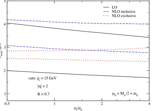
First full NLO calculations were published in 2006 [28]. Events with b jet pair in the final state were selected, with momentum of the dijet system pT >15 GeV and a pseudorapidity less than 2. Results were shown for two categories, inclusive and exclusive, depending on the treatment of extra jets. In the inclusive case events with additional jets were included, while in the exclusive case exactly two jets were required. Figure2.10shows the overall scale dependence of LO, NLO inclusive and NLO exclusive total cross-sections, when both renormalization scale and factorization scale are varied independently between
µ0/2 and 4µ0 (with µ0 = mb +MW/2), including full bottom-quark mass e↵ects. NLO
cross sections have a reduced scale dependence over most of the range of scales shown, and the exclusive NLO cross-section is more stable than the inclusive one especially at low scales. The e↵ect of the b quark mass has been shown to a↵ect the total NLO cross section on the order of approximately 8%. This is expected to be small when considering well separated jets.
checked that our implementation of the kT jet algorithm coincides with the one in MCFM.
We require all events to have a b¯b jet pair in the final state, with a transverse momentum
larger than 15 GeV (pb,T¯b >15 GeV) and a pseudorapidity that satisfies|⌘b,¯b|<2. We impose
the same pT and |⌘| cuts also on the extra jet that may arise due to hard non-collinear real
emission of a parton, i.e. in the processes W b¯b+g orW b¯b+q(¯q). This hard non-collinear
extra parton is treated either inclusively or exclusively, following the definition of inclusive
and exclusive as implemented in the MCFM code [25]. In the inclusive case we include
both two- and three-jet events, while in theexclusive case we require exactly two jets in the
event. Two-jet events consist of a bottom-quark jet pair that may also include a final-state light parton (gluon or quark) due to the applied recombination procedure. Results in the massless bottom-quark approximation have been obtained using the MCFM code [25].
0.5 1 2 4 µf/µ0 1 2 3 4 5 σtotal (pb) LO NLO inclusive NLO exclusive cuts: pt > 15 GeV |η| < 2 R = 0.7 µ0 = Mw/2 + mb
FIG. 4: Dependence of the LO (black solid band), NLO inclusive (blue dashed band), and NLO
exclusive (red dotted band) total cross-sections on the renormalization/factorization scales,
includ-ing full bottom-quark mass e↵ects. The bands are obtained by varyinclud-ing bothµR and µF between
µ0/2 and 4µ0 (with µ0 =mb+MW/2).
In Figs. 4-6 we illustrate the renormalization and factorization scale dependence of the
LO and NLO total cross-sections, both in the inclusive and exclusive case. Fig. 4 shows
the overall scale dependence of both LO, NLO inclusive and NLO exclusive total
cross-7
Figure 2.10: Wbb NLO scale dependence[28]
Chapter 2. Theoretical overview New results published in 2007 explored in particular NLO corrections for events with W boson and two jets where at least one is b-tagged. It was shown that for LHC the correction factor is ⇡ 1.9. This paper was interesting in particular for its study of soft and collinear topologies, where two b quarks merge into one. Additionally, b quarks in the initial state were considered, giving rise to processes like bq ! W bq0 shown in figure
2.8. The parton distribution function for b quark needed to be determined perturbatively using DGLAP equations. Another approach is to consider a gluon in the initial state, which then splits to b¯b.
2.2.2.1 Double parton scattering
Multiple parton interactions happen due to the composite nature of the proton. Usually it is assumed that only one hard scattering occurs per bunch crossing. The probability of single parton interaction in hadron collisions is very small thus having two or more interactions is highly suppressed. However, sometimes it can happen that two such partons exist which results in two hard scatterings in the same collision. This phenomenon is called Double Parton Scattering (DPS) and is shown in Figure 2.11. In the framework of this thesis, two partons are responsible for the creation of a W boson and other two for creation of a pair of b jets.
Chapter 3:
W
+
b
-jets: Theory and Previous Measurements
Figure 3.7: Sketch of a double-parton process in which the active partons are
i
and
k
from one proton and
j
and
l
from the second proton. The two hard scattering
subprocesses are (
ij
!
ab
) and (
kl
!
cd
)
general expression, adapted to the
W
+
b
-jets case, is:
DPS
(
pp
!
W
+
b
+
X
) =
X
i,j,k,lZ
dx
1dx
2dx
01dx
02db
2 ik(x
1, x
2, b, µ
F)
jl(x
01, x
02, b, µ
F)
⇥
ij!W(
x
1x
02s, µ
2F)
kl!b+X(
x
2x
02s, µ
2F)
(3.3)
In this equation, the two parton-level cross-sections represent the independent
processes
ij
!
W
and
kl
!
b
+
X
. They are each calculated using pQCD, as
per-turbation series in
↵s
, in the same way as they would be calculated for a single hard
scattering. The
ik(x
1, x
2, b, µ
F) functions represent the
double parton distribution
functions
(DPDFs), describing the probability to extract partons
i
and
k
, with
re-spective momentum fractions
x
1and
x
2, from the same proton. The parameterb
, new
with respect to the standard PDFs, represents the separation between
i
and
j
, as well
as between
k
and
l
, in the transverse plane perpendicular to the proton momentum.
29
Figure 2.11: Double parton scattering
Chapter 2. Theoretical overview
Double parton scattering cannot be modeled in the framework of preturbative QCD, but it is approximated using simulations. The phenomenology of DPS starts from the assumption that factorization between the two hard processes is possible, as well as fac-torization between hard processes and proton kinematics. Cross sections for hard scatter-ings are computed separately for each pair of partons. However, instead of using regular parton distribution functions, a new set of distribution functions has been defined which are called Double Parton Distribution Functions (dPDFs). Factorized cross section for two hard processes A and B to happen in proton-proton scattering can be written as:
DP S (A,B) ⇠ X i,j,k,l Z dx1dx2dx01dx02d2b ij(x1, x2, b;Q1, Q2) ikA(x1, x01) B jl(x2, x02) kl(x01, x02, b;Q1, Q2) (2.3)
Parton level cross sections are denoted with ik, for hard process between partons i
and k, and jl for hard process between partonsj and l. These are the same as for single
parton scattering and are known for most of the processes of interest today. The quantity
ij(x1, x2, b;t1, t2) represents the double parton distribution function, which describes the
probability of finding a parton i with momentum fraction x1 at scale Q1 inside a proton
together with a parton j with momentum fraction x2 at scale Q2. Another parameter
in this distribution function is b, which describes the transverse distance between two partons. The scales Q1 and Q2 and correspond to characteristic scales of hard processes
A and B. For example in the framework of this thesis the W boson production would correspond to process A and production of two b jets would correspond to process B. This study is described in detail in [29]. Usually, it is assumed that ij(x1, x2, b;t1, t2) can
be decomposed into two components, longitudinal and transversal in the following way:
ij(x1, x2, b;t1, t2) =Dijh(x1, x2;t1, t2)Fji(b) (2.4)
The interpretation of the function Dhij(x1, x2;t1, t2) within QCD is the probability of
find-ing partoniwith scale Q1 and partonj with scaleQ2. These functions cannot be
determ-ined using perturbative QCD. To make an accurate cross section predictions it is essential 22
Chapter 2. Theoretical overview to have good modelling and to correctly take into account the correlations between lon-gitudinal momenta and transverse position.
More details on how to determine dPDFs can be found in [30]. In the simplest case
Dijh(x1, x2;t1, t2) can be taken as a product of single parton distribution functions taking
into account e↵ects like x1+x2 <1. Since Fji(b) is the only part of (DP SA,B) that depends
only on b, integration over b can be performed giving an e↵ective cross section ef f which
is related to the size of the proton and can be seen as an e↵ective area of the interaction. This approach yields a simplified expression for the double parton scattering cross section:
DP S (A,B)⇠ 1 ef f SP S (A) (SP SB) (2.5) Here SP S
(A) and SP S(B) are single parton scattering cross section which can be obtained using
equation 2.2.
However, this factorized approach does not take into account some simple correla-tions, e.g. between the probability to find a quark of some flavor and to find find another quark with the same flavor. While for some simple cases with low parton momentum fractions this factorized approach may give accurate results, for more complicated cases like calculating fiducial cross sections, acceptance cuts can spoil the equation. Thus, a simulation of the full kinematical e↵ects is necessary.
A first measurement of ef f has been performed by the AFS collaboration at the
ISR (CERN) which obtained ef f ⇠5 mb at 63GeV. Both CDF and D0 collaborations at
Tevatron, Fermilab (IL, USA) reported ef f ⇠ 15 mb which is roughly 20% of the total pp¯cross section at Tevatron energies. Their data also show no sign of dependence on x
in measured ef f in the accessible x ranges. Later measurements performed by ATLAS
ans CMS collaborations are in reasonable agreement with previous results. All results are summarized in Figure 2.12.
Double parton scattering measurement at CMS is performed by selecting events with
Chapter 2. Theoretical overview
4
by the speakers on behalf of their collaboration.
In general these new experimental results, that show a
progress in the comprehension of the relevant systematic
uncertainties in particular for what concerns the
back-ground modeling, confirm the overall picture of
signifi-cant DPS rates at the LHC and lay the groundwork for
further DPS studies at the LHC, also in the light of
un-derstanding unexpected backgrounds in the search for
new physics.
In the future, the proposal of much higher center of
mass energies (HE-LHC) opens up the possibility to
study extreme kinematic regions of QCD that are still
not explored. The dynamics of the high energy limit of
QCD is driven by the increasingly higher gluon densities
at low parton fractional momenta, which should be
dom-inated by multiple parton interactions. With the future
high luminosity phase (HL-LHC) it will be possible to
achieve very clear evidence of DPS production focusing
on the final states with two heavy bosons, in particular on
the production of equal sign W boson pairs decaying
lep-tonically, leading to final states with same-sign isolated
leptons plus missing energy.
B.
DPS in W + 2-jet final states with CMS at the
LHC
We present a study of DPS based on W + 2-jet events
in pp collisions at 7 TeV using CMS detector [32]. DPS
with a W + 2-jet final state occurs when one hard
in-teraction produces a W boson and another produces a
dijet in the same pp collision. The W + 2-jet process is
attractive because the muonic decay of the W provides
a clean tag and the large dijet production cross section
increases the probability of observing DPS. Events
con-taining a W + 2-jet final state originating from single
parton scattering (SPS) constitute an irreducible
back-ground. Events with W bosons are selected requiring the
muon and missing transverse energy information. We
also select two additional jets with
p
T>
20 GeV/c
and
|
⌘
|
<
2.0.
We use two uncorrelated observables; the relative
p
T-balance between two jets (
relp
T) and azimuthal angle
between the W-boson and dijet system (
S). The
dis-tributions of the DPS-sensitive observables for the
se-lected events are corrected for selection efficiencies and
detector e↵ects, and compared with distributions from
simulated events. Simulations of W + jets events with
madgraph
5 +
pythia
8(or
pythia
6) and NLO
pre-dictions of
powheg
2 +
pythia
6(or
herwig
6) describe
the data provided MPI are included, as shown in the top
panel of Fig. 1.
pythia
8 standalone fails to describe
data mainly in the DPS-sensitive region due to missing
higher order contributions.
To extract the DPS fraction, signal and background
templates are defined in such a way that signal and
back-ground events cover the full phase space. The fraction of
DPS in W + 2-jet events is extracted with a DPS + SPS
template fit to the distribution of the
S
and
relp
T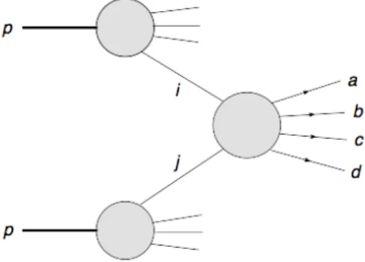
![Figure 3.2: Parton distribution functions at two di↵erent scales, Q 2 = 10 GeV and Q 2 = 10 4 GeV, as calculated by the MSTW group [57].](https://thumb-ap.123doks.com/thumbv2/123dok/1321076.2511774/34.893.157.731.383.756/figure-parton-distribution-functions-erent-scales-calculated-mstw.webp)

![Table 3.1: LHC performance in 2012 together with design performance[ 41 ]](https://thumb-ap.123doks.com/thumbv2/123dok/1321076.2511774/53.893.155.738.370.554/table-lhc-performance-design-performance.webp)
![Figure 4.4: A drawing of the CMS strip detector. [ 37 ]](https://thumb-ap.123doks.com/thumbv2/123dok/1321076.2511774/62.893.159.736.438.702/figure-drawing-cms-strip-detector.webp)