Extract relevant features from DEM for groundwater potential mapping
Tao Liu a ,b,*,Haowen Yan a,b, Liang Zhai c a
Faculty of Geomatics, Lanzhou Jiaotong University, Lanzhou, China b
Gansu Provincial Engineering Laboratory for National Geographic State Monitoring, Lanzhou, China c
Key Laboratory of Geo-Informatics of National Administration of Surveying, Mapping and Geoinformation, Beijing, China
KEY WORDS: DEM; Groundwater potential; Multi-criteria evaluation (MCE); Area under curve (AUC); GIS
ABSTRACT:
Multi-criteria evaluation (MCE) method has been applied much in groundwater potential mapping researches. But when to data scarce areas, it will encounter lots of problems due to limited data. Digital Elevation Model (DEM) is the digital representations of the topography, and has many applications in various fields. Former researches had been approved that much information concerned to groundwater potential mapping (such as geological features, terrain features, hydrology features, etc.) can be extracted from DEM data. This made using DEM data for groundwater potential mapping is feasible. In this research, one of the most widely used and also easy to access data in GIS, DEM data was used to extract information for groundwater potential mapping in batter river basin in Alberta, Canada. First five determining factors for potential ground water mapping were put forward based on previous studies (lineaments and lineament density, drainage networks and its density, topographic wetness index (TWI), relief and convergence Index (CI)). Extraction methods of the five determining factors from DEM were put forward and thematic maps were produced accordingly. Cumulative effects matrix was used for weight assignment, a multi-criteria evaluation process was carried out by ArcGIS software to delineate the potential groundwater map. The final groundwater potential map was divided into five categories, viz., non-potential, poor, moderate, good, and excellent zones. Eventually, the success rate curve was drawn and the area under curve (AUC) was figured out for validation. Validation result showed that the success rate of the model was 79% and approved the method’s feasibility. The method afforded a new way for researches on groundwater management in areas suffers from data scarcity, and also broaden the application area of DEM data.
* Corresponding author.Email:[email protected]
1. INTRODUCTION
Groundwater is one of the most important natural sources (Lee, Kim et al. 2012, Haleh Nampak 2014, Rahmati, Nazari Samani et al. 2014). With the progressive evolution of human activity, the water demand continuously increases (Samy Ismail Elmahdy, 2014), which necessitates the planning of groundwater recharge (Tarun Kumar, 2014). Groundwater potential, which can be defined as the possibility of groundwater occurrence in an area (Rahmati, Nazari Samani et al. 2014), is becoming a hot research issue.
Traditional approaches for assessing groundwater potential is drilling, which is high costly. The advance of geographic information system (GIS) and remote sensing (RS) techniques has brought a more efficient way for groundwater potential mapping.
Researches have been done to prepare a groundwater potential map (Ratnakar Dhakate, 2008) using geomorphological and geophysical units which were interpreted from remote sensing data; GIS and RS techniques were used, geology and geomorphology factors were mainly took into account, Vanessa Madrucci(2008) presents the groundwater favorability mapping in brazil; Lithological and geomorphologic layers were integrated in GIS environment Imran A. Dar (2010) integrated GIS and RS to map groundwater potential zones ; Geographic information system (GIS) and a probability model was used , hydrological data was used , Hyun-Joo Oh(2011) studied the groundwater potential mapping in Korea. Related data such as topography and geology data was collected, Saro Lee (2012)
implemented the weights-of-evidence method for groundwater potential mapping; Geology, geomorphology and hydrology thematic layer were prepared by Tarun Kumar (2014) to generate the groundwater potential zone map.Terrain features, lithology, land use and soil hydrology factors were concerned, a statistical model was proposed by Moghaddam D. Davoodi(2015) for Groundwater spring potential mapping. Many researchers have found that multi-criteria evaluation (MCE) method is an effective tool for delineating groundwater potential resources. As mentioned above, all kinds of thematic layers and data were prepared for multi-criteria construction. When to data scarce areas, this method will encounter lots of issues due to the limited data.
Many studies have revealed that groundwater potential is related with many factors, such as geological features, terrain features, hydrology features, etc. Digital Elevation Model(DEM) is the digital representations of the topography, the technological advances provided byGIS and the increasing availability and quality of DEMs have greatly expanded the application potential of DEMs to many applications in many fields(Moore, Grayson et al. 1991).Among those factors related to groundwater potential mapping, most of the information has been proved can be extracted from DEM data, and this made extracting relevant features from DEM for groundwater potential mapping is feasible.
The main goal of this study is to delineate groundwater potential zones using DEM data, one of the most widely used and also easy to access data in GIS, provide a quick and low
expense methodology for groundwater potential mapping, and help to the decision makers in groundwater management.
2. STUDY AREA
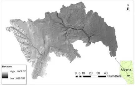
The study site was located in batter river basin in Edmonton-Calgary corridor, Alberta, Canada. The total area is 7256 (km2) The DEM data of the study area was obtained with 25m resolution, the lowest elevation is 680m and the highest elevation is 1008m, the mean elevation is 795m with the standard deviation of 65.5m. As figure 1 showed, the study site generally had higher elevation in the west area, lower elevation in the east. Noticed that there were several flat areas, they belonged to water body. These areas can be subtracted out as non-potential area.
Figure.1 DEM and location of the study area .
3. MAIN DETERMINING FACTORS
Groundwater potential is associate with many factors. According to the studies had mention before, this paper selected five main determining factors for groundwater potential modelling. They were lineaments density, drainage networks density; topographic wetness index (TWI), relief and convergence index (CI).These factors can be extracted from DEM data, and also were crucial for groundwater potential mapping.
3.1 Criteria 1: Lineament density
Lineaments (linear features), which were surficial expressions of underlying structural features like geological fractures( i.e. faults or joints in hard rock areas), indicating the occurrence of groundwater (Todd and Mays, 2005) and act as conduits of groundwater flow. They play a significant role in the occurrence and movement of groundwater(Mohamed 2014).Lineament density was calculated using total length of lineaments subtracted by unit area as equation (1) showed.
A
L
D
ni i
l
1 (1) Where
L
idenotes the lineament’s length
A
denotes the unit area
D
l denotes the lineament’s densityIt was assumed that the intensity of fracturing decreases with increasing distance away from the lineaments. This implies that the best chances for groundwater targeting are close to lineaments(Manika Gupta 2010).
Researches had done about extracting geology fractures from DEM. Guth(1999,2001) developed a topographic fabric algorithm by calculated flatness parameters and organization parameters. Also the MICRODEM freeware program was developed. As a first step, the algorithm needed 4 parameters to be input, they were point separation (in meters), regional size (in meters), flatness cut-off and length multiple.
Point separation was the distance between points at which the grain would be calculated. The higher this parameter was the less number of geographical fractures extracted. Regional size was the size of the blocks over which the fabric would be calculated. Too small region would not get reasonable statistics. Flatness cut-off was flatter points that would not be plotted. The larger the value selected, the more points would be plotted, but they might be subject to random noise (Guth 2001). The appropriate value depended in part of the scale of the DEM and the relief in the region. The fourth parameter length multiple was the scaling factor for length of fabric vectors. A higher value of length multiple would increase the length of geographical fractures extracted. The four parameters needed for running the algorithm was discussed in detail by Mohamed (Mohamed 2014) . In this research the MICRODEM freeware was used to generate geological fabrics (As shown in figure2a). After lineaments’ extraction, lineaments density map had been produced for the study area which was carried out by ArcGIS software (As shown in figure 2b).
.
Figure 2a. Geological fabrics extracted and aspect rose diagram
Figure 2b. Lineaments density map
3.2 Criteria 2: Drainage networks density
Many algorithms had been put forward on extracting drainage networks from DEM (Kiss 2004 ). The D8(deterministic eight-node) algorithm had widely used and implemented in ArcGIS
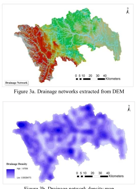
software(Mohamed 2014).In this paper we used the ArcGIS software(D8 algorithm) for drainage network extraction(As shown in figure 3a) .After extraction of drainage networks , drainage density map is produced for groundwater modelling. Drainage density can indicate the permeability of the area thus had close relation to groundwater potential mapping. Low drainage density indicates high permeable surface, while high drainage density indicates low permeable surface, which conversely tends to be concentrated in surface runoff. Drainage density is defined as the total length of the stream segments per unit area(N.S. Magesh 2012). Drainage density of the study area is calculated using line density analysis tool in ArcGIS software (As shown in figure 3b).
Figure 3a. Drainage networks extracted from DEM
Figure 3b. Drainage network density map 3.3 Criteria 3: TWI (Topographic wetness index)
The topographic wetness index (TWI) was commonly used to quantify topographic control on hydrological processes and reflects the potential groundwater exfiltration caused by the effects of topography, thus higher TWI value represented higher groundwater potential value. The index was a function of both the slope and the upstream contributing area per unit width orthogonal to the flow direction (Also called specific catchment area, SCA, m2.m-1). Its definition was as follow:
)
tan
ln(
TWI
(2)
Where '
' denotes the local upslope area draining through a certain point per unit contour length
Denotes slope angleA higher TWI indicated a gentler slope and larger slope area. The procedure yielded a suitable representation of divergent and convergent flow pattern in hilly terrains. However, in rather flat areas and particularly in broad valleys near the
talwegs, small differences in altitude caused random like flow pattern, which distinctly limit the predictive capacity of all related secondary terrain indexes in soil regionalization.
Figure 4a.
Cumulative percentage of slope
Figure 4b.
Slope map of study area
According to the cumulative percentage of slope figure and slope map (figure 4a and figure 4b), 95% slope is below 6(%), the study site basically belonged to plain area. The SAGA TWI, however, was based on a modified calculation of the catchment area, which assumed rather homogenous hydrological conditions in these flatter areas (Bohner& Selige, 2006), was applied in this research. Instead of using plain
, an iteration form of SCA (3) was used to calculate the Wetness Index (4).)
exp(
15
)
15
1
max(
SCA
M
SCA
For
)
15
exp(
)
15
1
max(
SCA
SCA
(3))
tan
ln(
M
SCA
TWI
(4)
Where SCA denotes the specific catchment area (m2.m-1)
Denotes the slope angleAccording to the formulas mentioned above, the Topographic Wetness Index was calculated in SAGA software and the result was as figure 5 shown.
Figure 5. TWI map of study area
3.4 Criteria 4: Relief
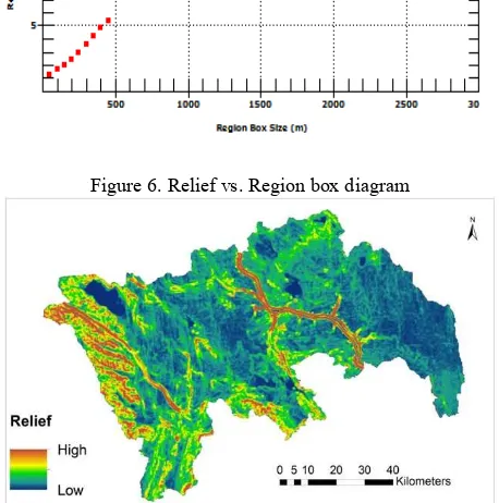
Relief played an important role in determining the infiltration rate of the rainfall, flow accumulation, transit and dissipation zone(Mohamed 2014).Areas with low relief was closed associated with groundwater accumulation. As the figure 6 shown, the relief of the study site was increased with increasing region box size because more points were considered. But there was a break of region box size at 600(m). When region box size was bigger than 600m, the relief was increased slowly with the box size increasing. So we calculated the relief 600(m) of the study site for analyzing, and the final relief 600(m) map was shown in figure7.
Figure 6. Relief vs. Region box diagram
Figure 7.Relief 600(m) map of study area 3.5 Criteria5: Convergence Index
Convergence Index (CI) was used to distinguish flow convergent area from divergent area(Kiss 2004 , N. Thommeret 2009), thus could be used for groundwater potential modelling.
CI could be calculated based on the aspect which can be extracted from DEM. The CI was obtained by calculating the average angle (ie. θ in figure 8a) between the aspect of adjacent cells and the direction to the central cell and then subtracts 90°.
Figure 8. (a) convergence index calculation; (b) CI equals -90°with θ is 0°;(c) CI equals 90°with θ is 180°; (d) CI equals
0°with θ is 90°
As the figure 8a shown, the convergence index was defined as:
90
8
1
81
i i
CI
(5)Where θ denotes average angle (ie. θ in figure 8a) between the aspect of adjacent cells and the direction to the central cell. The possible value ranged from -90°to +90°.As the figure 8b,8c,8d shown, they represented when the CI value equalled -90°, + 90°, 0°respectively. Positive CI values represented divergent area while negative CI values represented convergent area. Thus a lower CI value associated with groundwater accumulation and had a higher groundwater potential value. The CI map of the study area was shown in figure 9.
Figure 9. Convergence Index map of the study area
4. WEIGHT ASSIGNMENT
Weight assignment was an important part in potential groundwater modelling. Many studies implemented frequency ratio method (Ozdemir 2011a ,Mohammady et al. 2012; Ozdemir and Altural 2013), other studies described probabilistic model’s application (Murthy and Mamo 2009; Oh HJ et al. 2011). Logistic regression approach also was a frequently used method (Ozdemir 2011b). Basically these studies divided the drilling wells data into 2 parts, one part was used for training, and the other part was used for validation. This method was not applicable in data scarcity areas.
In this research, we used the cumulative effect matrix for weight assignment. For the mentioned five determine factors, we could construct a 5×5 matrix. If one factor had effect on the other, then the two factors’ conjunction point’s score would be 1, otherwise the score would be 0. For example, lineament density (Dl in table1) had effects on TWI, Drainage network density (Dd in table1) and CI but no effects on Relief, thus the effect score of Dl is 1, 1,0,1,1 respectively (factors had effects on itself, that’s why the diagonal line’s score was 1) .Then each factor’s cumulative effect was calculated, the weight was assigned by using each factor’s cumulative effect score divided the total cumulative effect score. The cumulative effect matrix and the weight assignment process were show in the table 1. The effect score was mainly obtained through expert knowledge and previous studies (N.S. Magesh, 2012; Samy Ismail Elmahdy, 2014).Noticed that the score on the diagonal line was assigned with 1.
Tab.1 Main Potential Groundwater Factors and Cumulative Effect matrix relief, and had the highest score which means had the biggest weight (31%). TWI and CI had the same score thus the same weight (23%), drainage network succeeded (15%), and relief factor had the least score and weight (8%).
5. POTENTIAL GROUNDWATER MAPPING AND VALIDATION
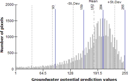
Using the DEM data prepared in section 2, five determining factors were extracted according to section 3. Using the weight assignment method in section 4, weighted overlay analysis was carried out by ArcGIS software. After mean filtering for smoothing image, the nature break ranking method (main break values are as shown in figure 10) was applied to obtain
the final groundwater potential map. The final groundwater potential map was divided into five categories, viz., non-potential, poor, moderate, good, and excellent zones.
Figure 10. Histogram of Groundwater potential prediction values & natural breaks values (blue line)
Figure11. Groundwater Potential map of the study area Result map shown that non-potential, poor, moderate, good, excellent areas were 2.6%, 19.8%, 39.4%, 29%, 9.2% of the total area respectively. The non-potential areas were mainly water body. The excellent and good potential groundwater area mainly lied in west area where geological fractures density was high. The poor potential groundwater area was located at east part of batter river basin where geological fractures density was low and drainage density was high.
Validation was carried out based on the Edmonton–Calgary Corridor groundwater atlas (2011).Compare to the atlas’ potential groundwater map which based on the driller’s assessment of the sediment in which the well is completed, most of the excellent ,good and moderate zones obtained by the proposed method was coincide with the areas of atlas. Computation result shown that the map using the proposed method had a 77% accurate rate.
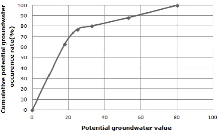
Additionally, by comparing and overlaying the obtained map with the wells data and potential groundwater map in the atlas, cumulative percentage of the groundwater occurrence were calculated. Then these data was plotted on x axis-cumulative percentage of potential groundwater value and y axis- cumulative percentage of groundwater occurrence. Then the success curve was obtained as figure 12 shown. Area under curve (AUC) was calculated to describe the accuracy of the obtained map. The AUC was 0.79 which corresponded to 79% of success accuracy. This validation result was almost the same with the accurate rate when comparing to the atlas.
Figure 12.The success rate curve of groundwater potential map 6. CONCLUSION
Multi-criteria evaluation (MCE) method had been proved a valid method in groundwater potential mapping researches. This paper concentrated on areas suffering from data scarce issues when to apply MCE method. DEM data, one of the most widely and easy to access data was used, five determining factors/criteria was extracted from DEM first, and then cumulative matrix was used for weight assignment. Weighted overlay analysis was applied by ArcGIS software according to the weight assigned. Mean filter was applied to achieve noises’ cut down and image smooth, finally the natural break ranking technique was used to obtain the groundwater potential map. The final groundwater potential map was divided into five categories, viz., non-potential, poor, moderate, good, and excellent zones. The accuracy rate obtained by comparing to the groundwater atlas and by AUC analysis was 77% and 79% respectively. The validation result showed the feasibility of the method which was putted forward in this paper, and also broaden the application area of DEM.
ACKNOWLEDGEMENTS
This work was funded by national nature science foundation of china (grant no.41201476), china postdoctoral science foundation (grant no.2013M542397), Open foundation of Key Laboratory of Geo-Informatics of National Administration of Surveying, Mapping and Geoinformation(grant no.201409).
REFERENCES
Barker, A.A., Riddell, J.T.F., Slattery, S.R., Andriashek, L.D., Moktan, H., Wallace, S., Lyster, S., Jean, G., Huff, G.F., Stewart, S.A. and Lemay, T.G., 2011. Edmonton–Calgary Corridor groundwater atlas; Energy Resources Conservation Board, ERCB/AGS Information Series 140, 90 p.
Bohner, J., Selige, T., 2006. Spatial prediction of soil attributes using terrain analysis and climate regionalisation. SAGA–Analyses and Modelling Applications.–Göttinger Geographische Abhandlungen, 115:13-28.
Guth, P.L.1999. Quantifying and Visualizing Terrain Fabric from Digital Elevation Models: in Diaz, J., Tynes, R., Caldwell, D., and Ehlen, J., eds., Geocomputation 99: Proceedings of the 4th International Conference on GeoComputation, Fredericksburg, Virginia, USA, 25-28 July, 1999.
Guth, P.L. 2001. Quantifying terrain fabric in digital elevation models, in Ehlen, J., and Harmon, R.S., eds., the environmental legacy of military operations, Geological Society of America Reviews in Engineering Geology, vol, 14, chapter 3, p.13-25
Haleh Nampak, B. P., Mohammad Abd Manap, 2014. Application of GIS based data driven evidential belief function model to predict groundwater potential zonation. Journal of Hydrology, 513: 283-300.
Kiss, R. 2004. Determination of drainage network in digital elevation models, utilities and limitations. Journal of Hungarian geomathematics, 2: 22-36.
Lee, S., Y. S. Kim and H. J. Oh , 2012. Application of a weights-of-evidence method and GIS to regional groundwater productivity potential mapping. Journal of Environmental Management ,96(1): 91-105.
Manika Gupta , P. K. S., 2010. Integrating GIS and remote sensing for identification of groundwater potential zones in the hilly terrain of Pavagarh, Gujarat, India. Water International 35(2): 233-245.
Mohamed, S. I. E. M. M. 2014. Groundwater potential modelling using remote sensing and GIS: a case study of the Al Dhaid area, United Arab Emirates. Geocarto International 29(4): 433-450.
Mohammady M, Pourghasemi HR, Pradhan B ,2012 Landslide susceptibility mapping at Golestan Province, Iran: a comparison between frequency ratio, Dempster–Shafer, and weights of evidence models. Journal of Asian Earth Science, 61:221–236
Moore, I. D., R. B. Grayson and A. R. Ladson ,1991. Digital terrain modelling: A review of hydrological, geomorphological, and biological applications. Hydrological Processes, 5(1): 3-30. Murthy KSR, Mamo AG ,2009. Multi-criteria decision evaluation in groundwater zones identification in Moyale– Teltele subbasin,South Ethiopia. International Journal of Remote Sensing, 30:2729–2740
N. Thommeret, J. S. B., C. Puech ,2009. Robust Extraction of Thalwegs Networks from DTMs for Topological Characterisation: A Case Study on Badlands. Proceedings of Geomorphometry 2009. Zurich, Switzerland, 31 August - 2 September, 2009: 218-223.
N.S. Magesh, N. C., John Prince Soundranayagam ,2012. Delineation of groundwater potential zones in Theni district, Tamil Nadu, using remote sensing, GIS and MIF techniques. Geoscience frontiers, 3(2): 189-196.
Oh HJ, Kim YS, Choi JK, Lee S, 2011. GIS mapping of regional probabilistic groundwater potential in the area of Pohang City,Korea. Journal of Hydrology, 399:158–172 Ozdemir, A. 2011a. GIS-based groundwater spring potential mapping in the Sultan Mountains (Konya, Turkey) using frequency ratio, weights of evidence and logistic regression methods and their comparison. Journal of Hydrology, 411: 290-308.
Ozdemir,A. 2011b. Using a binary logistic regression method and GIS for evaluating and mapping the groundwater spring potential in the Sultan Mountains (Aksehir, Turkey). Journal of Hydrology, doi:10.1016/j.jhydrol.2011.05.015
Ozdemir A, Altural T ,2013. A comparative study of frequency ratio,weights of evidence and logistic regression methods for landslide susceptibility mapping: Sultan Mountains, SW Turkey. Journal of Asian Earth Science, 64:180–197
Rahmati, O., A. Nazari Samani, M. Mahdavi, H. Pourghasemi and H. Zeinivand, 2014. Groundwater potential mapping at Kurdistan region of Iran using analytic hierarchy process and GIS. Arabian Journal of Geosciences: 1-13.
Tribe, Andrea, 1992. Automated recognition of valley lines and drainage networks from grid digital elevation models: a review and a new method. Journal of Hydrology 139.1: 263-293. Turcotte, R., et al.,2001. Determination of the drainage structure of a watershed using a digital elevation model and a digital river and lake network. Journal of Hydrology 240.3 : 225-242.
Wechsler, S. P. 2007. Uncertainties associated with digital elevation models for hydrologic applications: a review, Hydrology. Earth System. Science, 11:1481-1500,