www.elsevier.comrlocateratmos
A parameterization of cloud microphysics for
long-term cloud-resolving modeling of tropical
convection
Wojciech W. Grabowski
National Center for Atmospheric Research,1Boulder, CO 80307, USA
Received 15 March 1999; received in revised form 17 May 1999; accepted 7 June 1999
Abstract
This paper documents development of a simple cloud microphysical parameterization for use in long-term cloud-resolving simulations of maritime tropical convection. The parameterization is
Ž .
based on the bulk approach and considers two classes of liquid water cloud water and rain and
Ž .
two classes of ice slowly falling ice A and fast-falling ice B . Ice A represents unrimed or lightly rimed ice particles whose spectral characteristics are assumed to follow aircraft observations in tropical upper-tropospheric anvil clouds. Ice B, on the other hand, represents heavily rimed ice
Ž .
particles e.g., graupel which occur in the vicinity of convective towers. Mixing ratios for these four classes of cloud condensate are used as model variables. Together with the mixing ratio for water vapor, five field variables are used to represent all forms of water in the tropical atmosphere. The parameterization is used in a prescribed flow model to illustrate development of tropical convective and stratiform precipitation. Application of the parameterization to the cloud-resolving simulations of cloud systems observed during the TOGA COARE field campaign is also presented.q1999 Elsevier Science B.V. All rights reserved.
Keywords: Cloud modeling; Cloud microphysics; Tropical convection
1. Introduction
The increase of computational resources in recent years enables application of cloud models to problems directly related to the role of clouds in the climate system. This is especially relevant for the Tropics because diabatic effects associated with cloud processes can only be crudely captured in large-scale models, which have to rely on sub-gridscale parameterizations. Cloud-resolving simulations with spatial resolutions of
1
The National Center for Atmospheric Research is sponsored by the National Science Foundation. 0169-8095r99r$ - see front matterq1999 Elsevier Science B.V. All rights reserved.
Ž .
Ž
;1 km are able to consider tropical cloud systems in large computational domains up
5 2. Ž
to 10 km and to study their evolution over extended periods of time up to several weeks, see Grabowski et al., 1996 and references therein; Grabowski et al., 1998; Wu et
.
al., 1998, 1999, among many others . This approach is referred to as cumulus ensemble Ž .
modeling, or a cloud-resolving modeling CRM approach.
Representation of cloud microphysics in cloud models applied in such long-term simulations is arguably one of the major uncertainties of the CRM approach. The role cloud microphysical processes play in such simulations has been recently documented
Ž . Ž .
by Wu et al. 1999 and, in more general terms, by Grabowski et al. 1999 . Because the CRM approach is computationally very demanding, it is unlikely that sophisticated approaches which consider details of the evolution of cloud condensate from very small water or ice particles up to precipitation-size particles can be included. Consequently, simple microphysical parameterizations, employing as few field variables as possible to represent cloud condensate, and firmly based on cloud observations, should be the
Ž .
starting point. This is the approach advocated by Grabowski 1998 . It can also be Ž
argued that there is still not enough known about cloud microphysics ice physics in .
particular for trustworthy comprehensive parameterizations to be designed for use in climate-related cloud-resolving studies. From that perspective, a simple approach which includes as few tunable parameters as possible and at same time is capable of capturing the essential aspects of cloud microphysics, seems very appealing.
The purpose of this paper is to present a microphysical scheme that has been developed for long-term CRM of tropical convection. The emphasis is on cloud microphysics at cold temperatures, that is, involving the ice phase, because
upper-tropo-Ž spheric ice clouds have an important effect on radiative processes in the tropics e.g.,
.
Ramanathan and Collins, 1991 . In addition, traditional ice schemes used in cloud models are based on spectral characteristics of ice particles obtained in extratropical
Ž .
cloud systems either convective or stratiform . As far as the ice microphysics is concerned, the scheme proposed herein follows a strategy suggested by Koenig and
Ž . Ž .
Murray 1976 hereinafter KM76 . It considers two classes of ice, referred to as ice A Ž and ice B for which only conservation equations for mixing ratios are considered KM76 solved for both mixing ratios and number concentrations of ice A and ice B in their
.
approach . Ice A represents slowly falling ice particles produced by diffusional growth of pristine ice crystals. Its spectral characteristics are based on aircraft observations of
Ž
upper-tropospheric tropical ice clouds McFarquhar and Heymsfield, 1997, hereinafter
. Ž .
MH97 . Ice B, on the other hand, represents heavily rimed ice particles graupel which Ž . in the proposed scheme originate from the interaction of ice A with rain KM76 . These two mechanisms of precipitation formation are thought to mimic development of
Ž .
2. The parameterization
As discussed in Section 1, the approach is designed to capture essential aspects of the cloud microphysics using as few model variables as possible. As far as warm-rain
Ž .
processes are concerned, an approach similar to Kessler 1969 is used, that is, mixing ratios for the cloud water and for the rain water are predicted. In addition, mixing ratios for the two classes of ice, referred to as ice A and ice B, are considered. Altogether, four model variables are designated for four classes of the cloud condensate. The equations describing the moist precipitating thermodynamics are as follows:
Er uo
and qB are the cloud water, rain water, ice A, and ice B mixing ratios. The sinks and sources due to microphysical transfer terms are depicted as FF; the sedimentation
velocities for the rain, ice A, and ice B are V , V , and V , respectively, and k is ther A B
unit vector in the vertical direction. Other symbols and constants are listed in Appendix Ž . Ž . Ž . Ž . Ž . Ž .
B. Note that, in general, Eqs. 1a , 1b , 1c , 1d , 1e and 1f should include Ž
additional terms on the right-hand-side e.g., due to subgrid-scale turbulence parameteri-.
Ž . Ž . Ž . Ž . Ž . Ž . The sourcesrsinks of water substance in Eqs. 1a , 1b , 1c , 1d , 1e and 1f describe phase changes and they are parameterized based on the following assumptions Žsee Appendix A for details . Cloud water is formed when the air becomes supersatu-. rated with respect to water. The condensation instantaneously brings the air back to saturation. The cloud water moves with the air and evaporates instantaneously in undersaturated conditions. The cloud water is a source of rain. Rain moves relative to the air, collects cloud water as it falls through the cloud, and can evaporate in the undersaturated conditions outside clouds. Raindrops are assumed to follow the size
Ž .
distribution of Marshall and Palmer 1948 with the prescribed intercept and the slope dependent upon the rain mixing ratio. When temperatures fall below freezing, ice A
Ž
forms due to either heterogeneous or homogeneous for temperatures colder than .
y408C nucleation of ice crystals. The heterogeneous nucleation rate depends on the availability of ice-forming nuclei, which in the current formulation depends on the air temperature alone. Ice A particles are assumed to follow size distributions observed in
Ž .
upper-tropospheric tropical anvil clouds MH97 . MH97 consider two separate size distributions for small and large ice particles and such an approach is included in the parameterization of ice A. Interaction of ice A with raindrops results in formation of ice B which is assumed to have Marshall–Palmer type size distribution typical for graupel
Ž .
particles as in Rutledge and Hobbs 1984 . Growth of either ice A or ice B particles is represented by the parameterization developed by KM76 which relates the ice particle
Ž
growth rate by either water vapor diffusion or accretion of supercooled liquid water, or .
both to environmental conditions. Both ice A and ice B move relative to the air with sedimentation velocities depending on the ice mixing ratio and the air density. Upon crossing the melting level, ice A and ice B melt and are converted into rain.
Ž . Ž . Ž . Ž . Ž . Ž . The microphysical water transfer terms in Eqs. 1a , 1b , 1c , 1d , 1e and 1f
Ž
describe the following processes the sink and the source of the water are shown in the .
parentheses : Ž .
Ø COND qv™q : condensation of water vapor to form cloud water;c
Ž . Ž .
Ø AUTC qc™q : autoconversion of cloud water into rain initiation of the rain field ;r
Ž .
Ø RCOL qc™q : collection of cloud water by rain water;r
Ž .
Ø REVP qr™q : evaporation of rain;v
Ž . Ž .
Ø HETA qc™qA : heterogeneous nucleation of ice A freezing of cloud droplets ;
Ž .
Ž . Ž . Ž . Ž . Ž . The treatment of the sources and sinks on the rhs of Eqs. 1a , 1b , 1c , 1d , 1e
Ž . Ž .
and 1f is similar to that used by Grabowski and Smolarkiewicz 1996 : only condensa-Ž tion is treated to the second order in time and all other sources apply uncentered i.e.,
.
first order in time approach.
Because of the finite time step, sourcesrsinks of water variables can result in Ž . negative values of a condensate variable. A simple solution is to limit the lhs of Eq. 1c as
approach results in a lack of conservation of total water and energy, as the adjustment Ž .2 affects only a sink of one variable and not the corresponding source of another
Ž .
variable in the system 1 . To ensure conservation of water and energy, the adjustment Ž2a is supplemented with the adjustment of the water vapor and temperature sources. according to:
The model applies accurate formulations for the saturated water vapor pressure over water and over ice for a wide range of ambient temperatures. Tables of the saturated vapor pressure with respect to water and ice are created during model startup using
Ž .
accurate but expensive formulas discussed by Flatau et al. 1992 . The tables provide saturated vapor pressure using the temperature interval of 0.1 K. Linear interpolation using the tabulated values is applied during model run to deduce the saturated vapor pressure for a given temperature.
w Ž . Ž . y1x
Fig. 1. Horizontal velocities thin lines, solid dashed for positive negative values, contour interval 3 m s
Ž y1.
3. Kinematic framework tests
Ž .
Prescribed flow simulations Szumowski et al., 1998 represent an attractive way of testing microphysical parameterizations before they are used in a dynamic model. In
Ž . Ž . Ž . Ž . Ž . Ž .
tests presented in this paper, Eqs. 1a , 1b , 1c , 1d , 1e and 1f is solved using a Ž .
two-dimensional x–z flow prescribed to mimic development of either convective or
Ž .
stratiform precipitation Houze, 1997 . In the former case, precipitation develops mostly due to accretional growth of water and ice particles, whereas diffusional growth of the ice phase dominates in the latter one. The tests illustrate that the parameterization is capable of reproducing these two modes of precipitation development.
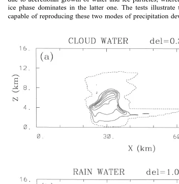
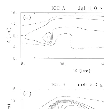
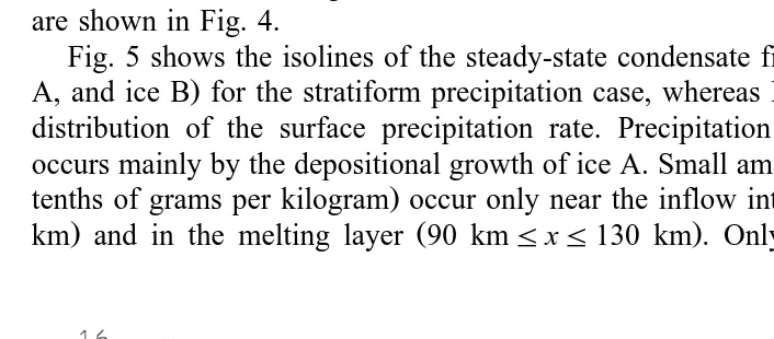
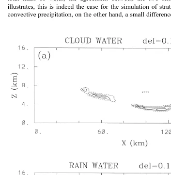
Fig. 2. Isolines of the condensate fields for the kinematic test mimicing development of convective
Ž . Ž . Ž . Ž .
precipitation at time ts4 h. The panels show cloud water a , rain b , ice A c and ice B d mixing ratios
y1Ž . y1 Ž . y1Ž .
with contour intervals of 0.2 g kg a , 1.0 g kg b, c , and 2.0 g kg d . The dashed contours are for mixing ratios of 0.01 g kgy1
Ž .
Fig. 2 continued .
The initial temperature and moisture profiles are taken from the 00 GMT September
2 Ž
1st, 1974 GATE sounding applied in simulations described by Grabowski et al. 1996, .
1998, 1999 . These profiles are also used on inflow lateral boundaries. Zero-gradient conditions are applied on lateral outflow boundaries. The advection is performed using a
Ž .
monotone MPDATA algorithm Smolarkiewicz and Margolin, 1998 and 15-s time step is used in the calculations. The simulations are carried out for 4 h for the convective situation and for 8 h for the stratiform situation, which are sufficient to established steady-state thermodynamic fields inside the domain.
2
w Ž . x
In the convective precipitation case, the computational domain is 90 km long and 16 km deep with a uniform grid of size of 500 m in the horizontal dimension and 250 m in
Ž the vertical. The flow is prescribed using a steady streamfunction given by cf.
. Grabowski, 1998
ro pz
ˆ
pxˆ
1 2C
Ž
x , z.
sA sinž / ž /
sin y SzŽ .
3roo Z X 2 where As4.8=104 kg my1 sy1, S
s2.5=10y2 kg my3 sy1, r
s1 kg my3, oo
Ž . Ž Ž ..
zs
ˆ
min z, Z , xˆ
smaxyX,min X, xyxc , Zs15 km, Xs10 km, xcs30 km, and Ž w x w x.x, z are the coordinates which cover the entire domain i.e., 0, 90 km= 0, 16 km . The streamfunction provides a narrow zone of the lifting throughout the entire
tropo-Ž
sphere centered at xc with corresponding low-level convergence and upper-level .
divergence superimposed with the vertical shear of the horizontal wind which allows mean advection of the rising air from the left to the right of the domain. The velocity
Ž .
components are deduced from Eq. 3 as rous yECrEz and rowsECrEx and they
are shown in Fig. 1. The updraft speed reaches a maximum of about 7.5 m sy1
at a height of about 7.5 km.
Ž
Fig. 2 shows the isolines of the steady-state condensate fields cloud water, rain, ice .
A, and ice B for this case, whereas Fig. 3 shows the horizontal distribution of the
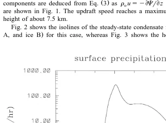
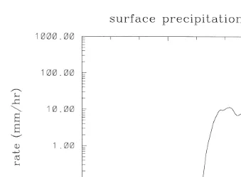
Fig. 3. Distribution of the surface precipitation intensity in mm hy1 across the domain at time ts4 h for the
surface precipitation rate. As shown in Fig. 2, precipitation development occurs through the conversion of cloud water into rain in the lower part of the updraft, and through
Ž .
growth of the graupel ice B field above. The trace of cloud water extends as high as 11 km, which is approximately the level at which the temperature drops belowy408C and homogeneous nucleation becomes possible. Fig. 2 also documents an extensive anvil cloud formed by the horizontal advection of ice A from the convective updraft. The horizontal distribution of surface precipitation shows high values for the precipitation intensity, a characteristic of convective rainfall, giving way to more moderate intensities as one moves downstream from the location of the strong updraft.
In the stratiform precipitation case, the computational domain is chosen as 180 km long and 16 km deep with a uniform grid of size of 1000 m in the horizontal and 250 m in the vertical. In this case, the flow is prescribed using a streamfunction pattern
ro 2 pz
ˆ
pxˆ
C
Ž
x , z.
sA sinž /
sinž /
yQzŽ .
4roo Z1 X
4 y1 y1 y2 y1 Ž Ž ..
with As4=10 kg m s , Qs3 kg m s , z
ˆ
smin Z ,max 0, z1 yZ2 ,Ž Ž ..
xs
ˆ
maxyX,min X, xyxc , Z1s10 km, Z2s3 km, Xs70 km, and xcs72 km. The streamfunction provides a wide zone of gentle lifting superimposed with a weak flow across the domain flow from left to right. The updraft speed reaches a maximum of about 0.8 m sy1 at a height of about 8 km. The horizontal and vertical velocity isoplethsare shown in Fig. 4.
Ž
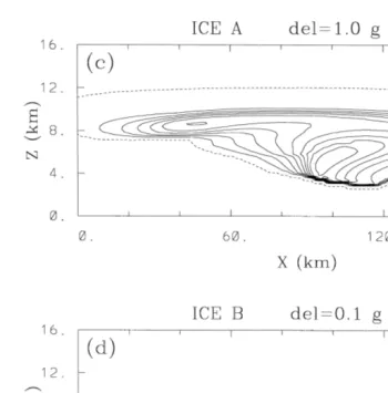
Fig. 5 shows the isolines of the steady-state condensate fields cloud water, rain, ice .
A, and ice B for the stratiform precipitation case, whereas Fig. 6 shows the horizontal distribution of the surface precipitation rate. Precipitation development in this case
Ž occurs mainly by the depositional growth of ice A. Small amounts of cloud water a few
. Ž
tenths of grams per kilogram occur only near the inflow into the updraft zone z;60
. Ž .
km and in the melting layer 90 kmFxF130 km . Only traces of the ice B field
Žgraupel are present. Consequently, surface precipitation rates Fig. 6 are between 1. Ž . and 10 mm hy1 which are typical for stratiform precipitation.
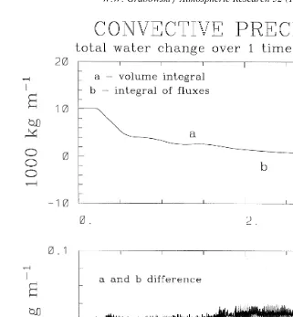
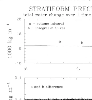
Water conservation in the kinematic framework simulations is illustrated in Figs. 7 and 8. The figure compares time step-by-time step changes of the volume-integrated
Ž .
total water a sum of the water vapor and all forms of the condensate with the total flux Ž
of water across the domain boundaries see Section 4 of Szumowski et al., 1998 for .
details . In the case when both advection and microphysical adjustments conserve the total mass of water, the agreement between the two should be perfect. As Fig. 8 illustrates, this is indeed the case for the simulation of stratiform precipitation. For the convective precipitation, on the other hand, a small difference between the two estimates
Fig. 5. As Fig. 2, but for the kinematic test mimicing development of stratiform precipitation at time ts8 h.
Ž . Ž . Ž . Ž .
The panels show cloud water a , rain b , ice A c and ice B d mixing ratios with contour intervals of 0.1 g
y1Ž . y1Ž .
Ž .
Fig. 5 continued .
of the total water change develops in the second half of the simulation. However, the difference is comparable to the fluctuations of the total water calculation due to roundoff errors which are apparent as fluctuations in the bottom panels of Figs. 7 and 8.
4. Application to the tropical convective systems during TOGA COARE
The parameterization of moist precipitating thermodynamics described in this paper
Ž w x
was applied to the GCSS GEWEX Global Energy and Water-Cycle Experiment Cloud
. Ž .
Fig. 6. As Fig. 3, but for the kinematic test mimicing development of stratiform precipitation at time ts8 h.
The numerical model is the two-time-level, nonhydrostatic Eulerianrsemi-Lagrangian Ž .
anelastic fluid model EULAG of Smolarkiewicz and Margolin 1997 . The Eulerian version of the model is used. The 2D computational domain is 800 km long and 30 km deep with a uniform grid with 2 km resolution in the horizontal direction and 0.3 km resolution in the vertical. The time step is 10 s. The large-scale advective tendencies of
Ž .
the temperature and moisture usually referred to as large-scale forcing terms as well as Ž .
the evolution of horizontal winds and the sea surface temperature SST are prescribed Ž .
to the model based on the Intensive Flux Array IFA observations. The dynamic model Ž .
includes the TOGA COARE surface flux algorithm of Fairall et al. 1996 with the cool-skin and warm-layer corrections omitted for simplicity. The NCAR Community
Ž .
Climate Model radiation code Kiehl et al., 1994 is used for radiative transfer calculations which are performed every 10 min of model time. Cloud water and ice A are the only forms of condensate used as input into the radiation code. The effective radius reff of condensate particles is assumed as 10 mm for cloud water and for ice A
Ž .
the effective radius is expressed as a function of the ice water content IWC based on the aircraft observations of MH97:
log r10 effsaX2qbXqc
Ž .
5Ž 3 . Ž y3 . Ž .
where Xslog10 10 IWC IWC in kg m , reff inmm and the coefficients in Eq. 5
y2 Ž .
Ž
Fig. 7. Comparison between changes of the total water expressed as a mass of water in a unit distance in the y1.
third spatial direction, i.e., in kg m during the model time step derived from the total water inside the
Ž . Ž
domain upper panel, solid line and derived from the total water fluxes across the model boundaries upper
.
panel, dashed line for the kinematic tests mimicing development of convective precipitation. The lower panel shows the difference between the two derivations of the total water change.
and 140 mm are used for IWC smaller than 10y4 g my3 and larger than 1 g my3,
respectively.
Ž .
Fig. 9 shows the Hovmoller
¨
x–t diagram of the surface precipitation rate to illustrate the organization and movement of convection. During the 5-day simulation, three periods of strong convection are separated by two periods of little or no convection. The movement of the surface precipitation from east to the west in the first 2 days and from west to east in the second half of the simulation match the results ofŽ . Ž . Wu et al. 1998 Fig. 7 .
Fig. 8. As Fig. 7, but for the kinematic test mimicing development of stratiform precipitation.
. see also the WG4 website at htpp:rrwww.met.utah.edurskruegerrgcssrwg4.html The approximately 2 K difference between the model results and observed temperature
Ž profiles is a subject of an ongoing investigation of the GCSS WG4 community an error in the imposed large-scale forcing terms may be the culprit, see discussion in Krueger
.
and Lazarus, 1999 . The deviation in the moisture field is likely a result of the missing Ž
large-scale advective tendencies of cloud condensate Grabowski et al., 1996, 1998; Wu .
et al., 1998 .
Ž . Finally, Fig. 11 shows the evolution of the outgoing longwave radiation OLR and
Ž . 3
the top-of-the-atmosphere TOA albedo as predicted by the numerical model and the
w Ž
estimates of these quantities based on the satellite observations the ISCCP International
3 Ž
The TOA albedo is defined as the ratio between the net solarflux at the top of the atmosphere i.e.,
.
Ž .
Fig. 9. Hovmoller x – t diagrams for the surface precipitation rate for the simulation of the TOGA COARE¨
convection. Precipitation intensity larger than 1 and 10 mm hy1 is shown using light and dark shading,
respectively.
. Ž .
Satellite Cloud Climatology Project Flux Cloud FC dataset for TOGA COARE, see
x
Burks and Krueger, 1999 and references therein . The evolution of the OLR follows in Ž
Fig. 10. Profiles of the 5-day mean difference between the model results and the observations for the temperature, the water vapor mixing ratio and the relative humidity for the simulation of the TOGA COARE convection.
Fig. 11. Evolution of the domain-average OLR and the TOA albedo for the simulation of the TOGA COARE
Ž .
.
Lazarus, 1999; Wu et al., 1999, Fig. 1 with the values for periods with weak or no convection in excess of 250 W my2, and values smaller than 150 W my2 for periods of strong convection. However, it seems that the model tends to overpredict the OLR and to underpredict the TOA albedo, at least when compared to the FC data.
5. Concluding remarks
This paper documents a simple microphysical scheme designed for long-term cloud-resolving modeling of tropical convection. The scheme uses a traditional bulk approach
Ž .
for warm rain physics Kessler, 1969 and considers two paths of precipitation develop-ment associated with ice physics. These two paths are related to the two modes of tropical rainfall: the convective mode, associated with accretional growth rain and ice,
Ž and the stratiform mode, dominated by the depositional growth of the ice field e.g.,
.
Houze, 1997 . Consequently, two classes of ice field are considered: ice A, representing unrimed or lightly rimed ice crystals, and ice B, representing the heavily rimed particles Žgraupel . The ice A is assumed to have spectral characteristics of ice particles observed.
Ž .
in upper-tropospheric tropical anvil clouds McFarquhar and Heymsfield, 1997 . The formation and growth of the ice field is represented using a simplified approach of
Ž . Koenig and Murray 1976 .
Ž
The parameterization is applied in tests with prescribed flow cf. Szumowski et al., .
1998 which illustrate development of convective and stratiform precipitation. These tests also document conservation of water mass by the microphysical scheme. The Fortran code for these tests is available from the author and can be applied to any microphysical scheme to document its performance. The microphysical scheme is also applied to the TOGA COARE convection and is shown to produce results consistent with other cloud-resolving models.
Acknowledgements
Greg McFarquhar kindly provided details of the CEPEX aircraft observations used in the derivation of terminal velocities and effective radii of ice particles. Changhai Liu provided assistance with the satellite data shown in Fig. 11. Comments on the manuscript by Changhai Liu and Roy Rasmussen are acknowledged, as is the editing of the manuscript by Jim Pasquotto. This work is supported by NCAR’s Clouds in Climate
Ž .
Program CCP . The National Center for Atmospheric Research is operated by the University for Atmospheric Research under sponsorship of the NSF.
Appendix A
The microphysical transfer terms are derived using estimates of particle concentra-tions and growth rates as given by assumed particle size distribuconcentra-tions and environmental
Ž .
Ž .
and d mArd t dep are estimates of ice A particle concentration and the depositional growth rate of an ice A particle, respectively. The SI units are used throughout the Appendix unless otherwise stated.
Ž .
Raindrops follow the size distribution of Marshall and Palmer 1948 with the constant intercept N0r and the slope lr given by
0 .25
prwN0 r
lrs
ž
/
Ž
A.1.
roqr
where rw is the water density. It follows that the mean concentration n , the mean sizer Drs2 R , and the mean mass m of raindrops, can be estimated asr r The raindrop terminal velocity is assumed to depend on its diameter D as Õ D s
r
0.5 Ž .
130 D Kessler, 1969 . The mass weighted terminal velocity V of the rain field isr
0 .5
where the reference air density in the last factor of Eq. A.3 is taken as 1 kg m . Ž .
Parameterization of ice B graupel is similar to the formulation for rain and follows Ž .
Rutledge and Hobbs 1984 . Ice B particles are also assumed to follow the size Ž .
distribution of Marshall and Palmer 1948 with the constant intercept N0B and the slope
lB
0 .25
prBN0 B
lBs
ž
/
Ž
A.4.
roqB
where rB is the graupel density. As in the rain case, the mean concentration n , theB
mean size DBs2 R , and the mean mass mB B of ice B particles can be estimated as
N0 B 1 prB
nBs , DBs , mBs 3 .
Ž
A.5.
lB lB 6lB
The terminal velocity of an ice B particle is assumed to depend on its diameter D as
Ž . 0.37 Ž .
ÕB D s19.3 D Rutledge and Hobbs, 1984 . Consequently, the mass weighted
terminal velocity VB of the ice B field is
0 .5
1
y0 .37
VBs31.2lB
ž /
.Ž
A.6.
ro
The formulation for ice A follows discussion in MH97. Based on in-situ aircraft observations, MH97 concluded that the ice particles in the upper tropospheric anvil clouds follow two separate size distributions: the first-order gamma distribution
describ-Ž .
observed IWC and parameters of the distributions in terms of the ambient temperature. The contribution of the IWC content due to small crystals IWC is approximated asS
0 .837
y3 y4 3
IWCSsmin 10
ž
,roq , 2.52A =10Ž
10roqA.
/
Ž
A.7.
y3 Ž .
where a limit of 1 g m is imposed on the maximum IWC in the case when Eq. A.7S
is applied to ice A mixing ratios higher than observed by MH97. The average mass of a small ice A paticle mAS is calculated as
2prI
mASs a3
Ž
A.8.
whererI is the ice density and a is the parameter of the first-order gamma distribution ŽEq. 6 in MH97 :.
4 3 4 3
asmax 2.2=10 ,y4.99=10 y4.94=10 log10
Ž
10 IWCS.
Ž
A.9.
and the minimum value of a corresponds to an ice particle with a melted diameter of 100mm. The mass-weighted terminal velocity of small ice A particles VAS is assumed
y1 Ž .
constant VASs0.1 m s G. McFarquhar, personal communication . The average mass of a large ice A particle mAL is calculated as
9
17 2
mALs1.67=10 prIexp 3
ž
mq s/
Ž
A.10.
2
Ž
where m and s are the parameters of the lognormal distribution Eqs. 7 and 8 in .
where TCsTy273.16 is the temperature in8C. The mass-weighted terminal velocity of large ice A particles VAL is estimated based on the aircraft observations discussed in
Ž .
MH97 G. McFarquhar, personal communication :
V s0.9q0.1log
Ž
103IWC.
Ž
A.14.
AL 10 L
Ž .
where dsIWCSr roqA is the relative contribution of the small IWC and the
Ž . y3
reference air density in the last factor of Eq. A.15b is taken as 0.3 kg m . When the
Ž . Ž . Ž .
ice particle size D or terminal velocity Õ as a function of the ice particle mass m is
Ž Ž ..
needed for instance, to estimate the particle Reynolds number, see Eq. A.25 , formulas representing rough fits to the observational data in the form ms2.5=10y2D2
0.25 Ž .
and Õs4 D Grabowski, 1988; Grabowski, 1998 are used.
Ž . Ž . Ž . Ž . Ž . Ž .
The water transfer terms in Eqs. 1a , 1b , 1c , 1d , 1e and 1f are calculated in the following way.
Ø The condensation term COND is defined by the requirement to maintain saturated Ž
conditions with respect to the plane surface of water cf. Grabowski and Smolarkiewicz, .
1990, 1996 .
ØThe autoconversion term AUTC is calculated using an approach proposed by Berry Ž1968 and applied by Simpson and Wiggert 1969. Ž . ŽSection 3 and Grabowski 1998. Ž .
where nc is the concentration of cloud droplets expressed in number per cubic .
centimeter and d is the relative dispersion of cloud droplet spectrum, i.e., the ratioc between standard deviation of cloud droplet spectrum and the mean droplet radius.
Ž .
Simpson and Wiggert 1969 suggested that the relative dispersion changes from 0.366 for maritime clouds with n s50 cmy3 to 0.146 for continental clouds with n s2000
c c
cmy3. The relative dispersion is calculated from the prescribed n and the two extreme c
which gives the relative dispersion of 0.33, 0.26 and 0.19 for droplet concentrations of 100, 300 and 1000 cmy3.
ØCollection of cloud water by rain RCOL is calculated using a continuous collection equation for a mean raindrop:
d mr N0 r 2 2roq Nc 0 r
RCOLsnr s pRrÕr
Ž
Rr.
Erroqcs5.78=10Ž
A.17.
7r2
ž /
d t col lr lrwhere E is the collection efficiency.r
1r2 Ž Ž .
where Fs0.78q0.27R is the ventilation factor R sDÕ D ry is the Reynolds
r e e r r r
. Ž . y7 XŽ . y7Ž Ž . 2 .y1
number , G Te s10 G Te s10 2.2Teresw Te q2.2=10 rTe , and Ss qvrqvsw is the saturation ratio.
Ø The heterogeneous nucleation of ice A HETA is assumed to occur through the freezing of cloud droplets. It occurs when the ice A mixing ratio is smaller than the mixing ratio obtained from the concentration of ice nuclei at a given temperature and the
Ž y1 2
mass of the ice A particle assuming it cannot be smaller than 10 kg which .
corresponds to a droplet with about 10 mm diameter . For computational reasons, the nucleation occurs over a finite time scale tn, where tn can be specified equal to the model time step Dt. The formula is
X
temperature alone and it is given by Fletcher, 1962 :
N T smin 105, 10y2
exp 0.6DT A.20
Ž .
Ž
Ž
.
.
Ž
.
IN
Ž .
where DTs273.16yT and the maximum concentration 100 per liter is imposed to
prevent unrealistically high concentrations in the upper troposphere where homogeneous nucleation dominates. If appropriate, another formulation for NIN can easily be included.
Ø The homogeneous nucleation of ice A HOMAsHOMA1qHOMA2 occurs only for temperature colder than 233.16 K. It transfers all cloud water and part of the water Ž . vapor into the ice A category; see discussion in Appendix B of Grabowski et al. 1996 . The formulae are
qv and qv denoting the saturated mixing ratios with respect to water and ice, and the sw si
Ž
coefficient b depends on the temperature it decreases linearly from bs1 for Ts
. 233.16 K to bs0.1 for TF213.16 K, cf. Grabowski et al., 1996, Appendix B .
Ø Heterogeneous nucleation of ice B HETBsHETBqHETB2 occurs as a result of collisions between raindrops and ice A particles when the temperature is below freezing. The transfer terms are calculated using an estimate of the rate of collisions based on mean sizes and terminal velocities. The rate of collisions NrA per unit volume between raindrops and ice A is based on the continuous collection model and it is approximated as
N0 r 2roqA
< <
NrAs VryVApRr
Ž
A.22.
and the transfer terms are given by
HETB1sN m , HETB2rA r sN mrA A
Ž
A.23.
Ž .
Ø Growth of ice A and ice B particles by deposition of water vapor DEPA, DEPB
Ž . Ž .
and by riming RIMA, RIMB is calculated as described in KM76 Section 2 . In general, the growth rate of a single ice particle is prescribed based on the particle size
Ž
and environmental conditions such as temperature, supersaturation, and the amount of .
cloud water and rain available for growth by riming, see Fig. 2 in KM76 . An important aspect of the KM76 parameterization is that the diffusional growth of an ice particle at a given supersaturation is allowed to depend on the environmental temperature. Conse-quently, the parameterization attempts to represent dependence of the depositional growth rate of ice particles on the particle habit. As far as the growth by riming is concerned, it is assumed to occur through the interactions between ice A and the cloud
Ž . Ž . Ž .
water RIMA , whereas both cloud water via RIMB1 and rain via RIMB2 are considered for the growth by riming of ice B. The growth by riming is taken as a
Ž .
difference between the total growth as given by regimes A–B–C–D in Fig. 2 of KM76
Ž .
and the diffusional growth A–E in Fig. 2 of KM76 . With the growth of a single particle derived, the change of the mixing ratios are derived as:
roqA d mA
Note that Eqs. A.24a and A.24c are also applied to calculate the sublimation of ice A and ice B particles in undersaturated conditions.
Ž .
Ø Melting of ice A and ice B MELA, MELB for temperatures above freezing is a source of rain. Ignoring the evaporation andror sublimation of a melting particle, the
Ž . Ž
rate of the melting d mrd t me lt may be approximated as Pruppacher and Klett, 1978, .
Section 16.7, Rasmussen et al., 1984, Section 5 :
d mA 4pKa
s y DADTFA
Ž
A.25.
ž /
d t melt LfwhereDTs273.16yT and F s0.78q0.27R1r2 is the ventilation factor. The melting
A e
Appendix B
Below is a list of symbols and model coefficients used in the parameterization. The units andror values of a given symbol are given in the parenthesis.
Roman symbols
a , am s parameters in the formulation of m and s dependence on IWC and temperature
b , bm s parameters in the formulation of m and s dependence on IWC and temperature
Ž y1 y1. cp specific heat at constant pressure 1005 J kg K
dc dispersion of the cloud droplet spectrum
Ž .
D, D , D , Dr A B diameter, diameter of rain, ice A, ice B particle m
e , esw si saturation water vapor pressure with respect to water and Ž .
ice Pa
Ž .
Er collection efficiency for rain collecting cloud water 0.8 Ž
F , F , Fr A B ventilation factor for rain, ice A and ice B 0.78q 1r2.
0.27Re
G, GX thermodynamic functions in the formula for raindrop Ž y7 X.
evaporation Gs10 G
Ž y2 y1 y1 y1. Ka thermal conductivity of air 2.4=10 J m s K
L , L , Lv s f latent heat of evaporation, sublimation, and freezing Ž2.50=10 , 2.836 =10 , 3.36 =10 J kg5 y1.
m, m , m , mr A AL, mAS, mB mass, mass of a raindrop, mass of an ice A particle, mass of a large ice A particle, mass of a small ice A particle,
Ž . mass of an ice B particle kg
Ž y3. nc concentration of cloud droplets 200 cm
Ž y3. n , n , nr A B concentration of raindrops, ice A, ice B particles m
Ž y3. NIN concentration of ice nuclei m
NrA rate of collisions per unit volume between raindrops and Ž y3 y1.
ice A particles m s
N , N0r 0B intercept of the Marshall–Palmer distribution for raindrops Ž 7 6 y4.
T, T , T ,e C DT temperature, ambient profile of the temperature, tempera -Ž .
qv , qv saturated mixing ratio with respect to water and ice kg sw si
y1.
kg
Ž y1.
Õ terminal velocity of a single precipitation particle m s
V , V , Vr A AL, V , VAS B mass-weighted fall velocity of rain, ice A, large ice A, Ž y1.
Greek symbols
Ž y1.
a parameter in the small ice crystals size distribution m
b temperature-dependent coefficient in the formulation of the homogeneous nucleation of ice A
d the relative contribution of small ice A particles to the total ice A water content
u, ue potential temperature, ambient profile of the potential Ž .
temperature K
lr, lB slope of the Marshall–Palmer distribution for raindrops Ž y1.
and graupel m
m parameter in the lognormal distribution of large ice crys-tals
Ž y5 2 y1.
n kinematic viscosity of air 2=10 m s
Ž y3.
ro anelastic base state profile of the air density kg m
rw, rI, rB density of water, density of ice, density of ice B particle Ž 3 2 2 y3.
10 , 9=10 , 4=10 kg m
s parameter in the lognormal distribution of large ice crys-tals
Ž .
tn time scale of the ice A nucleation s
References
Berry, E.X., 1968. Modification of the warm rain process. In: Proceedings of the First National Conference on Weather Modification, Albany, NY, April 28–May 1, American Meteorological Soc., pp. 81–85. Burks, J.E., Krueger, S.K., 1999. Radiative fluxes and heating rates during TOGA COARE over the Intensive
Flux Array. Preprints, 23rd Conf. on Hurricanes and Tropical Meteorology, Dallas, TX. Am. Meteorol. Soc., pp. 773–775.
Fairall, C.W., Bradley, E.F., Rogers, D.P., Edson, J.B., Young, G.S., 1996. Bulk parameterization of air–sea fluxes for tropical ocean-global atmosphere coupled-ocean atmosphere response experiment. J. Geophys. Res. 101, 3747–3764.
Flatau, P.J., Walko, R.L., Cotton, W.R., 1992. Polynomial fits to saturation vapor pressure. J. Appl. Meteorol. 31, 1507–1513.
Fletcher, N.H., 1962. Physics of Rain Clouds. University Press, 386 pp.
Grabowski, W.W., 1988. On the bulk parameterization of snow and its application to the quantitative studies of precipitation growth. Pure Appl. Geophys. 127, 79–92.
Grabowski, W.W., 1998. Toward cloud resolving modeling of large-scale tropical circulations: a simple cloud microphysics parameterization. J. Atmos. Sci. 55, 3283–3298.
Grabowski, W.W., Smolarkiewicz, P.K., 1990. Monotone finite difference approximations to the advection-condensation problem. Mon. Weather Rev. 118, 2082–2097.
Grabowski, W.W., Smolarkiewicz, P.K., 1996. On two-time-level semi-Lagrangian modeling of precipitating clouds. Mon. Weather Rev. 124, 487–497.
Grabowski, W.W., Wu, X., Moncrieff, M.W., 1996. Cloud resolving modeling of tropical cloud systems during phase III of GATE: Part I. Two-dimensional experiments. J. Atmos. Sci. 53, 3684–3709. Grabowski, W.W., Wu, X., Moncrieff, M.W., Hall, W.D., 1998. Cloud resolving modeling of tropical cloud
systems during phase III of GATE: Part II. Effects of resolution and the third spatial dimension. J. Atmos. Sci. 55, 3264–3282.
Houze, R.A. Jr., 1997. Stratiform precipitation in regions of convection: a meteorological paradox?. Bull. Am. Meteorol. Soc. 78, 2179–2196.
Kessler, E., 1969. On the distribution and continuity of water substance in atmospheric circulations. Meteorol.
Ž .
Monogr. 10 32 , 84.
Kiehl, J.T., Hack, J.J., Briegleb, B.P., 1994. The simulated Earth radiation budget of the National Center for Atmospheric Research community climate model CCM2 and comparisons with the Earth Radiation Budget
Ž .
Experiment ERBE . J. Geophys. Res. 99, 20815–20827.
Koenig, L.R., Murray, F.W., 1976. Ice-bearing cumulus cloud evolution: numerical simulation and general comparison against observations. J. Appl. Meteorol. 15, 747–762.
Krueger, S.K., Lazarus, S.M., 1999. Intercomparison of multi-day simulations of convection during TOGA COARE with several cloud-resolving and single-column models. Preprints, 23rd Conf. on Hurricanes and Tropical Meteorology, Dallas, TX. Am. Meteorol. Soc., pp. 643–647.
Marshall, J.S., Palmer, W.McK., 1948. The distribution of raindrops with size. J. Meteorol. 5, 165–166. McFarquhar, G.M., Heymsfield, A.J., 1997. Parameterization of tropical cirrus ice crystal size distributions
and implications for radiative transfer: results from CEPEX. J. Atmos. Sci. 54, 2187–2200. Pruppacher, H.R., Klett, J.D., 1978. Microphysics of Clouds and Precipitation. Reidel, 714 pp.
Ramanathan, V., Collins, W., 1991. Thermodynamic regulation of ocean warming by cirrus clouds deduced from observations of the 1987 El Nino. Nature 351, 27–32.
Rasmussen, R.M., Levizziani, V., Pruppacher, H.R., 1984. A wind tunnel and theoretical study on melting behavior of atmospheric ice particles: III. Experiment and theory for spherical ice particles of radius)500 mm. J. Atmos. Sci. 41, 381–388.
Rutledge, S.A., Hobbs, P.V., 1984. The mesoscale and microscale structure and organization of clouds and precipitation in midlatitude cyclones: XII. A diagnostic modeling study of precipitation development in narrow cold-frontal rainbands. J. Atmos. Sci. 41, 2949–2972.
Simpson, J., Wiggert, V., 1969. Models of precipitating cumulus towers. Mon. Weather Rev. 97, 471–489. Smolarkiewicz, P.K., Margolin, L.G., 1997. On forward-in-time differencing for fluids: an
Eulerianrsemi-Lagrangian nonhydrostatic model for stratified flows. Atmos. Ocean Special 35, 127–152.
Smolarkiewicz, P.K., Margolin, L.G., 1998. MPDATA: a finite-difference solver for geophysical flows. J. Comput. Phys. 140, 459–480.
Szumowski, M.J., Grabowski, W.W., Ochs, H.T. III, 1998. Simple two-dimensional kinematic framework designed to test warm rain microphysical models. Atmos. Res. 45, 299–326.
Wu, X., Grabowski, W.W., Moncrieff, M.W., 1998. Long-term behavior of cloud systems in TOGA COARE and their interactions with radiative and surface processes: Part I. Two-dimensional modeling study. J. Atmos. Sci. 55, 2693–2714.