A long-term study of soil heat flux under a forest canopy
J. Ogée
∗, E. Lamaud, Y. Brunet, P. Berbigier, J.M. Bonnefond
INRA, Laboratoire de Bioclimatologie, BP 81, 33883 Villenave d’Ornon Cedex, France Received 29 March 1999; received in revised form 21 August 2000; accepted 1 September 2000Abstract
International programmes such as EUROFLUX focus on the analysis of long-term fluxes and energy budgets in the bio-sphere. Reliable estimates of hourly energy budgets require an accurate estimation of soil heat flux, that is often non-negligible even in a forest, and can be predominant during the night. Over long periods of time such as one to several months, its contri-bution can also be significant. The present work has been carried out to get good estimates of the soil heat flux in a maritime pine stand in the southwest of France, one of the 15 EUROFLUX sites. Using a whole year’s worth of data, soil heat flux was estimated by a two-step version of the null-alignment method using soil temperature, water content and bulk density measurements between the soil surface and a depth of 1 m. A data subset was firstly used to estimate and model the soil thermal conductivity at various depths. The full data set was then used with the modelled conductivity to estimate heat storage between the surface and a reference depth, and calculate the heat flux at the soil surface. Throughout the investigated year and at a 30 min time scale, the soil heat flux represents 5–10% of the incident net radiation, i.e. 30–50% of the net radiation over the understorey. Cumulative values from September 1997 to March 1998 reach a maximum of−70 MJ m−2, which represents
nearly 50% of the cumulative values of transmitted net radiation (140 MJ m−2) over the same period. These estimates of soil
heat flux allowed the energy budgets of the whole stand and the understorey to be closed, and showed that the storage terms are significant not only at a 30 min time scale but also at longer time scales (a few weeks). An attempt was finally made to model soil heat flux from meteorological data, which has rarely been done for a forest soil and over a long-term data set. In most of the existing models, soil heat flux is taken as a fraction of net radiation or sensible heat flux. Here, the litter acts as a mulch at the soil surface so that the only significant terms of the energy balance at this level are soil heat flux, transmitted net radiation and turbulent sensible heat flux. Soil heat flux is shown to be a linear combination of (1) net radiation above the understorey with a clear dependence of the coefficient on the soil cover fraction, and (2) the difference between the air and litter temperatures, with little influence of soil water content or wind speed on the coefficient. © 2001 Elsevier Science B.V. All rights reserved.
Keywords:EUROFLUX; Forest canopy; Long-term energy budget; Soil heat flux; Soil temperature; Understorey
1. Introduction
Recent developments in experimental techniques have allowed long-term continuous flux measurements of scalars such as heat, water vapour or CO2to be
per-∗Corresponding author. Tel.:+33-5-5684-3121;
fax:+33-5-5684-3135.
E-mail address:[email protected] (J. Og´ee).
formed over vegetation on a routine basis. Such mea-surements are a key feature in several international programmes, such as the European programme EU-ROFLUX, aimed at studying the role of the biosphere in global cycles.
As part of EUROFLUX, long-term eddy flux mea-surements of heat, water vapour and CO2have been
performed since July 1996 in a maritime pine forest in south western France. A major aim of this experiment
was to evaluate long-term energy budgets in order to understand how energy is shared, stored or released throughout the year between the pine trees, the under-storey and the ground. This is of particular interest in relatively open canopies with evergreen species like conifers: in such cases, the distribution of energy be-tween the trees and the understorey is likely to vary significantly through the year.
In this context, night-time and day-time periods are of equal interest since it is impossible to perform cu-mulative flux estimations without night-time values. As soil heat flux is a major term in the understorey energy budget during the night and a significant term in the day, a good estimation of this flux is critical in the context of long-term energy budgets.
For these reasons, soil heat flux measurements were performed continuously on our site. In the EU-ROFLUX programme, no recommendation was given about the method to be used for this. We designed an original method, well adapted to long-term measure-ments. It is derived from the null-alignment method of Kimball and Jackson (1975), that was further modi-fied to avoid its main drawbacks, as pointed out by de Vries and Philip (1986). This was made possible by the size of the data set collected during this exper-iment (nearly 17,400 temperature profiles recorded over almost 365 consecutive days are used here). Several tests validate this method in our context. In particular, estimated soil heat flux values allow the energy budgets of the whole stand and the under-storey to be closed (see Lamaud et al., 2000). Also, this large data set provides a good basis for modelling the soil heat flux from meteorological variables.
2. Experimental site and instrumentation
2.1. Experimental site
The experimental site is located at about 20 km from Bordeaux (44◦42′N, 0◦46′W, altitude 62 m) in a maritime pine stand (Pinus PinasterAit.) planted in 1970. The trees are distributed in parallel rows along a NE-SW axis. The inter-row distance is 4 m and the stand density is about 500 trees per hectare. The mean tree height is approximately 18 m. The under-storey mainly consists of grass (Molinia coeruleaL. Moench). The roots and the clumps remain throughout
the year but the leaves are green only from April to late November, with a maximum LAI and height of 1.45 and 0.7 m, respectively (Loustau and Cochard, 1991). In winter the soil is partly covered with dead leaves. A 5 cm thick litter layer made of compacted grass and dead needles is present all year long. The soil is a sandy and hydromorphic podzol, with a layer of pact sand located between 40 and 80 cm. The com-paction and chemical composition of this layer make it hardly penetrable by the roots, so that organic mat-ter is mainly located above it. During the 1997–1998 winter, the water table level went up to the soil sur-face. In summer, it was at a depth of about 120 cm.
2.2. Soil measurements
Soil temperature was measured at four different locations and eight depths: 1, 2, 4, 8, 16, 32, 64 and 100 cm using 32 home-made thermocouples, i.e. copper-constantan soldered joints coated with water-proof paint. All thermocouples had been previously tested in a thermally-regulated water bath for 48 h. Only those giving similar response curves were kept for our study. The leads were placed in plastic (PVC) tubes (2 cm in diameter) and the thermocouples were extracted at the measurement levels in such a way that their distance to the tubes was greater than 5 cm, in order to minimise the influence of conduction along the tubes. The portions of the leads remaining outside the tubes were then covered with heat-shrink tubing sheath. Insulation inside the tubes was in-sured by glue around the sheath. The four tubes were then inserted in the soil at four different locations as shown in Fig. 1. The thermocouples were con-nected to a multiplexer and the data was collected on a Campbell 21X data-logger (Campbell Scientific Ltd., Shepshed, UK). The measurements were made every 10 s and only half-hourly means were recorded. The data-logger temperature was used as the refer-ence temperature. Several checks using the amplitude differences and the phase shifts between the various levels showed that temperature measurements were accurate within±0.1◦C.
In this paper, we only use temperature values av-eraged over the four tubes. Standard deviations (not presented here) are always less than 0.5◦C and
av-erage around 0.1◦C. The data set covers the period
Fig. 1. Schematic representation of the site. Trees (closed circles) are aligned along a NE-SW axis with a 4 m inter-row distance. The triangles and the open circles represent the locations of soil temperatures profiles and soil humidity profiles, respectively.
profile is available every 30 min, except for a few hours in early March 1998 when the transmission system temporarily failed. Altogether we have about 17,400 temperature profiles.
Soil moisture was measured with a time domain reflectometer (TRASE systems, Soil Moisture Equip-ment Corp., Santa Barbara, CA) using 20 cm long buri-able waveguides. The latter were placed horizontally at three locations and four depths in the soil (5, 23, 34 and 80 m), and connected to a multiplexer (Fig. 1). The lower boundary (80 cm) coincides with the bot-tom of the root zone. The measurements were auto-matically recorded every 12 h. At each level humidity values were averaged over the three profiles. Battery problems caused occasional loss of data. A grand total of 229 midday profiles are used in this study.
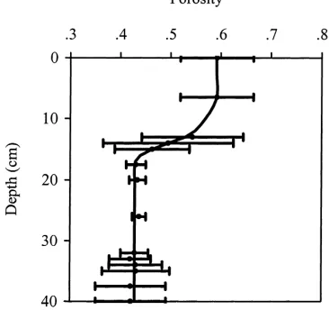
Profiles of soil bulk density had been previously measured by Diawara (1990) and more recently by Ar-rouays (personal communication). Soil samples from different depths and three locations in the vicinity of the other soil measurements were extracted, dried and weighed. Fig. 2 shows the mean profile of porosity over the top 40 cm, along with the standard deviation at each depth. Soil porosityεis related to bulk density,
ρ, by
ε=1− ρ
ρm
(1)
whereρm≈2660 kg m−3 is the density of minerals.
The experimental profile has been smoothed with a
Fig. 2. Profile of porosity,ε, in the top 40 cm: experimental data (closed circles) and adjusted profile with spline functions (solid line). The bars represent the standard deviations calculated over three experimental profiles.
spline function in order to get interpolates between the experimental points.
2.3. Micrometeorological measurements
Eddy fluxes of momentum, sensible heat, water vapour and CO2were measured above (and
occasion-ally below) the tree crown with the eddy-covariance technique. Heat storage in the air, the vegetation and the litter was also estimated using more than 60 thermocouples. All relevant details can be found in Lamaud et al. (2000). Above the canopy, at 25 m, global radiation was measured with a thermopile (Cimel CE 180, Paris, France) and net radiation was measured with a Q-7 net radiometer (Radiation En-ergy Balance System, Seattle, WA) that was viewing a representative area. Here also, samples were taken every 10 s, and 30 min means were recorded. The data was collected on a Campbell 21X data-logger.
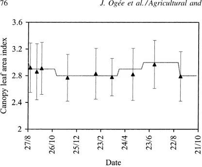
Fig. 3. Variation of mean canopy leaf area index during the ex-periment. Experimental data (triangles) and parameterisation used to calculate transmitted net radiation (solid line). The bars repre-sent the standard deviations calculated over a different number of points at each date.
temperatures. We use the litter temperature at the air-litter interface for the ground and the air tempera-ture at 14 m for canopy temperatempera-ture. The transmitted net radiation is then computed with
Rn,t=R′n,t+(1−f2)σ{Ta4,14m−Ta4,l} (2)
whereσ =5.67×10⁻⁸W m−2K−4,T
a,14mis the air
temperature at 14 m above ground, a surrogate for the mean foliage temperature,Ta,l is the air temperature
at the air-litter interface, andfandR′n,t are given by equations (9a) and (11a) of Berbigier and Bonnefond (1995), respectively.
The mean canopy leaf area index was measured reg-ularly by an optical method based on the interception of the solar beam (Lang, 1987). We observed contin-uous variations from about 2.8 in winter to almost 3.0 in summer (Fig. 3). The standard deviations shown in Fig. 3 are a consequence of the heterogeneity of the canopy rather than measurement uncertainties: at a given time of the year, different days of measurement would provide almost the same means and standard deviations.
3. Methodology
Several methods have been suggested to estimate the ground heat flux at the surface from
tempera-ture, humidity and bulk density data. A review can be found in Kimball and Jackson (1979). Most of these methods require extra information such as the soil thermal conductivity at some depth, or a value of soil heat flux as measured with a flux plate. The ad-vantage of the null-alignment method (Kimball and Jackson, 1975) is that no additional measurement is needed.
3.1. The null-alignment method (Kimball and Jackson, 1975)
We start with the continuity equation for heat (Kondo and Saigusa, 1994):
C∂T ∂t = −
∂Qh
∂z −LEsoil (3)
In this equation t is time (s), z the depth defined positive downwards (m), C the volumetric soil heat capacity (J m−3K−1), L the latent heat of
vaporisa-tion (J kg−1), T the local soil temperature (K), Q h
the downward soil heat flux (W m−2) and Esoil the
evaporation source strength ( kg m−3s−1). Integration of Eq. (3) betweenzand a reference depthzr, defined later, gives
The null-alignment method is based on two assump-tions, whose validity is discussed further: (1) the soil heat flux at the reference level is only transported by conduction and water vapour, which amounts to neglecting the transport of heat by the mass flow of liquid water, and (2) no evaporation occurs in the soil between the surface and the reference level. Assumption (1) leads to
whereλ(zr) is the effective soil thermal conductivity at the reference depth (W m−1K−1). Assumption (2)
Soil heat capacity can be estimated from (de Vries, 1963):
C=Cm(1−ε)+Cwθ
≈(2×(1−ε)+4.18×θ )×106 (7) whereCm ≈2 andCw ≈4.18 MJ m−3K−1 are the
heat capacities for minerals and water, respectively, and θ is soil volumetric moisture. In Eqs. (7) and (1), the organic matter is included with the minerals because it represents less than 5% in volume, even though its heat capacity and density are different from those of the minerals (Co ≈ 2.5 MJ m−3K−1
and ρo ≈ 1300 kg m−3 for organic matter). Hence,
from temperature, humidity and bulk density profiles, we are able to estimate all terms but the soil thermal conductivity at zr in Eq. (6). For this, the method
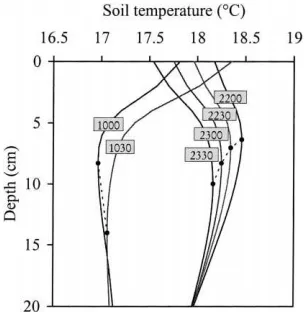
developed by Kimball and Jackson (1975) makes use of the fact that shortly after sunrise and sunset there is a well-defined level z0 near the surface (called ‘null-point’ by the authors), where the temperature gradient is zero (Fig. 4). Hence, for those times of the day when a null-point exists, Eq. (6) gives:
λ(zr)= +
timated several times a day (each time a null-point
Fig. 4. Temperature profiles at different times of the day on 4th of September (evening) and 23rd of September (morning) of year 1997. Time is indicated on each profile. Null-points are represented by closed circles. Temperature gradients below the null-point are positive downward in the morning, and positive upward in the evening.
occurred above the reference depth) and daily aver-ages were computed. These daily values of thermal conductivity were then used to compute the soil heat flux at any time of the day, assuming that λ(zr) did not change much throughout the day (Kimball and Jackson, 1975). In the present paper we adopt an-other scheme, that is better suited to long-term energy budget studies. It operates in two steps.
3.2. A two-step version of the null-alignment method
At a given depth the thermal conductivity is usually modelled as a function of temperature and volumetric moisture (de Vries, 1963). Such a parameterisation re-quires large ranges of soil moisture and temperature, that are normally encountered during a long-term ex-periment. In a first step, we use the whole data set and Eq. (8) (every time a null-point occurs) to estimate and modelλ(zr) as a function of soil volumetric moisture. Its temperature dependence is neglected. During the investigated year soil moisture ranges from dry values (5–6%) to saturation, providing us with the full range of variation of the thermal conductivity. In this first step, only the temperature profiles fulfilling the basic assumption of the null-alignment method are selected. In a second step, the whole data set is used again to calculate the heat flux throughout the year atzr, then
at the surface, using the modelled conductivity.
3.3. The reference depth zr
In the original version of the method the reference depth was chosen ‘shallow enough so that temperature changes can be measured accurately and deep enough so that thermal conductivity changes little during the day’ (Kimball and Jackson, 1975), and the authors rec-ommended zr = 20 cm. Here, the recommendations
should be similar because we also use daily estimates of soil thermal conductivity (from daily measurements of soil moisture). However, the main difference for the choice inzr is that our soil is covered by
10 cm (case A),zr=15 cm (case B) andzr =20 cm
(case C). The results are presented in Section 4.2.
3.4. Selection of temperature profiles to estimate soil thermal conductivity
As mentioned above, a selection was operated on the temperature profiles in order to satisfy the basic assumptions of the null-alignment method and get ac-curate estimates of the soil thermal conductivity.
According to the first assumption the heat trans-ported by the mass flow of liquid water must be negligible at the reference depthzr. This hypothesis
is not very restrictive and is often made for soil heat flux measurements (de Vries and Philip, 1986; Cellier et al., 1996) as well as in soil models (Kondo and Saigusa, 1994). As pointed out by de Vries and Philip (1986), ‘sensible heat transport produced by infiltra-tion of large quantities of water is potentially more important but this will occur through identifiable and anomalous events’, mainly during heavy rains. Hence, the temperature profiles recorded during heavy rains and within 2 h after them have been systematically removed from the set of profiles used to parameterise
λ(zr).
The second assumption of the null-alignment method states that no evaporation occurs between the null-point and the reference depth. This assump-tion is more stringent than the previous one and can in fact lead to unrealistic results if no precaution is taken (de Vries and Philip, 1986). In fact, if evapo-ration is not neglected, we obtain from Eqs. (4), (5) and (8):
where λna is the thermal conductivity derived from
the null-alignment method andQh,nathe
correspond-ing soil heat flux (previously denoted as λ and Qh, respectively). The temperature gradient at zr is posi-tive in the late morning, when evaporation is likely to
be positive, and negative in the late evening, when no evaporation (but rather condensation) occurs (Fig. 4). Therefore, in all cases, neglecting evaporation should lead to an underestimation ofλ:
λna(zr)≤λ(zr) (11)
The temperature gradient at 10 cm varies between
−20 and +20 K m−1. Hence, an evaporation of
2 W m−2, a reasonable value for a soil under a litter
and a canopy, would lead to an underestimation ofλ
of 0.1 W m−1K−1 if the null-pointz0 were so close
to the surface that all evaporation would occur below this level. This represents between 5 and 10% of the value ofλfor a sand with a medium range humidity. At other times of the day, when the temperature gra-dients are lower, the error could be more important. Fortunately, soil evaporation usually occurs only in the top centimetres. Hence, if the null-points are deep enough and if the gradients at the reference level are large enough, the conductivity estimates should be accurate. For this reason, we only selected temper-ature profiles with null-points deeper than 2 cm and temperature gradients larger than 4 K m−1. This is
in agreement with de Vries and Philip’s comments on the null-alignment method (de Vries and Philip, 1986).
Regarding now the computation of soil heat flux, it is highly desirable to keep as many values as possible, even during heavy rainfall or when soil evaporation is not a priori negligible. Our results show that the heat flux atzr only represents 20–30% of the surface flux, so that an error of 10% on the flux atzrwould lead to a 2–3% error on the flux at the soil surface, which is negligible in this type of energy budget studies. On top of this, soil evaporation is always very low in our con-ditions. At field capacity, when drainage is negligible (e.g. at the end of March 1998), the rate of decrease in soil moisture is of the order of−0.25 kg m−3d−1(not
3.5. Numerical implementation
All temperature profiles are smoothed using cubic splines (Press et al., 1992). They are used to interpolate the temperature at any depth, determine null-points and calculate temperature gradients at the reference depth (Fig. 4). Linear interpolation is used for humi-dity profiles because it was found that applying cubic splines to such profiles with few measurement depths can lead to unrealistic shapes.
Integrals in Eq. (8) (first step) and Eq. (6) (sec-ond step) are estimated using the trapezoidal rule. To avoid errors in the computation of the integral in Eq. (8), we also consider temperature profiles for which null-points are at 2 cm or more above the refer-ence levelzr. Hence, only 701 (case A:zr =10 cm),
1187 (case B: zr = 15 cm) and 1479 (case C:zr =
20 cm) of the 17,400 or so temperature profiles fulfil the conditions 2 cm≤z0≤(zr−2 cm)and∂T /∂z|zr
≥ 4 K m−1. Among them, only 458 (case A), 773 (case B) and 1085 (case C) profiles had been recorded during days when soil humidity was simultaneously measured. These profiles covered 237 (case A), 250 (case B) and 219 (case C) days, so that we had about 2 (case A), 3 (case B) and 5 (case C) profiles per day on average. Case C then had better statistics but covered fewer days than the other two cases. Case B covered a larger number of days with fewer profiles per day. The next section presents a comparison of the three cases.
4. Experimental results
4.1. Thermal conductivity versus soil volumetric moisture at three reference depths
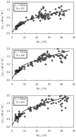
The experimentalλ–θ plots for the whole year and the three reference depths are presented in Fig. 5. Only mean daily values are plotted. The differences observed between the three sets of values reflect the spatial variations in bulk density that can be seen in Fig. 2.
These values are also compared with the model of de Vries (1963). To use it we assumed a quartz frac-tion of 95%, as suggested by Arrouays (personal com-munication), and a mean temperature of 285 K. The matric potential versus soil moisture curve required by the model was taken from Clapp and Hornberger
(1978) for our type of soil. The form factor ga was parameterised as in the original model (linear increase with moisture). Tests were also performed by adding a slight concavity in thega–θrelationship as suggested
by de Vries (1963). Because this made negligible improvement, no adjustment was made between the experimental data and the theoretical model. The vari-ations in bulk density allow the model to reproduce well the observed differences in thermal conductivity. The good agreement shows in particular that the selection made on the temperature profiles is correct. According to de Vries (1963), the model gives a typi-cal uncertainty of 5–10%, depending on the water status. Hence, the results are within the expected ex-perimental error. In what follows the soil heat flux is therefore computed using this model for λ, with the parameters described above.
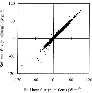
4.2. A comparison of soil heat fluxes using the three reference depths
Before choosing a reference level, it is desirable to compare the soil heat fluxes computed with various reference levels. A comparison is shown in Fig. 6. The computed values turn out to be similar over the whole range of soil moisture so that for the rest of the study only soil heat fluxes computed withzr =
10 cm are used, since this depth requires the smallest number of sensors. This result shows that an accurate computation of soil heat flux can be performed from temperature probes located in a shallow soil layer.
4.3. Half-hourly values
4.3.1. Annual variations of the daily cycle
All 17,400 or so 30 min temperature profiles are kept to compute the soil heat flux; for days when the soil moisture profiles were not recorded, linear inter-polation is performed between the preceding and fol-lowing values. Fig. 7a shows that the soil heat flux has a daily amplitude from about 25 W m−2in winter to more than 60 W m−2 in early summer, which rep-resents between 20 and 50% of the amplitude of the transmitted net radiation as can be seen in Fig. 7b. In this figure, the amplitude ofGhas been normalised by that ofRn,t to suppress the seasonal trend: these
Fig. 5. Soil thermal conductivity,λ(zr), vs. soil volumetric moisture,θ(zr), at three different depths,zr, (10, 15 and 20 cm): experimental
daily means (closed circles) and modelled curves (solid lines) using the model of de Vries (1963).
4.3.2. Energy budget
The energy budget closure is a good test to check whether or not flux measurements are correct. The soil is the most important sink or source of energy, as
Fig. 6. A comparison of soil heat fluxes computed withzr=10
andzr=20 cm for the full year of study (N=17,378 points). The
solid line is the linear regression line (R2=0.99, slope=1.01, intercept=0.57).
performed above the canopy. It was therefore possi-ble to evaluate the energy budget of each vegetation layer. The results are presented in a companion paper (Lamaud et al., 2000) which shows that the storage terms play an important role in the regulation of the energy cycle, especially in the understorey, and that the soil heat flux values obtained in the present work strongly improve the closure of the understorey en-ergy budget. Indeed, soil heat flux represents between 30 and 50% of transmitted net radiation at midday and up to 80% at night-time.
4.4. Daily values
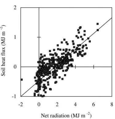
At a time scale of the order of one day or more, the soil heat flux is usually considered negligible on the basis that the heat stored during the day is released during the night. Indeed the daily sums of soil heat flux range between –1 and 1.5 MJ m−2during the pe-riod of study. Annual variations of these daily sums do not seem correlated with changes in soil moisture (not shown here), as is the case for daily amplitudes. However, they are linearly related to the daily sums of transmitted net radiation (Fig. 8). The negative value of the zero-intercept cannot be entirely attributed to an overestimation of the sky longwave radiation by
Fig. 7. (a) Maximum and minimum values of soil heat flux through-out the year of study: daily values (thin line) and 30-days moving averages (thick line). (b) Ratio of the daily amplitudes of soil heat flux,1G, and transmitted net radiation,1Rn,t, vs. near surface
soil moisture content.
the Q-7 net-radiometer as discussed in Berbigier et al. (2000) and probably has a physical origin.
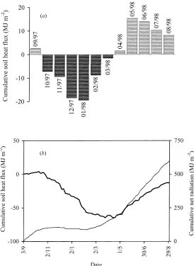
4.5. Monthly values
Monthly values of soil heat flux are presented in Fig. 9a. It can be seen that for long-term energy bud-get (one to several months), neglecting soil heat flux would generate an imbalance between turbulent fluxes and net radiation. From September 97 to March 98, the cumulative value of transmitted net radiation reaches about 140 MJ m−2(Fig. 9b). During the same period, the cumulative value of soil heat flux reaches a min-imum of−70 MJ m−2, i.e. 50% of the energy budget
Fig. 8. Daily sums of soil heat flux vs. daily sums of transmitted net radiation. The solid line is the linear regression line (R2=0.59, slope=0.27, intercept= −0.47).
5. Modelling soil heat flux
Models deriving soil heat flux from microclimatic measurements can be very useful, especially in the ab-sence of soil measurements. Several empirical models have been suggested to calculate the daytime heat flux in a bare soil from net radiation or sensible heat flux (Camuffo and Bernardi, 1982; Cellier et al., 1996). Some authors have studied how soil water content and mean wind speed may influence this type of relation (Idso et al., 1975). However, none of these models have been tested (1) under a forest canopy, (2) during night-time and (3) for yearly variations of the meteo-rological data and soil properties. The purpose of this section is then to find a simple parameterisation relat-ing the soil heat fluxG=Qh(0)to simple
microcli-matic data such as transmitted net radiation, and that would account for the seasonal variations in soil water content or soil cover fraction.
5.1. Soil heat flux and transmitted net radiation
Modelling soil heat flux from net radiation is not trivial because their relationship involves other fluxes through the energy budget equation. In the case of a soil under a forest canopy, the radiation hitting the ground must go through the canopy and the
under-storey. Hence, it exhibits strong horizontal heterogene-ity, which can only be appreciated at the expense of a heavy experimental set-up. As mentioned earlier net radiation above the understorey is estimated with a modified version of the radiative transfer model of Berbigier and Bonnefond (1995). Because we did not have a radiative transfer model for the understorey it-self, it was decided to use this flux in what follows.
We saw that the diurnal amplitude ofGis correlated toRn,t and soil water content (Sections 4.3 and 4.4).
We also observed that the maxima ofGandRn,t do
not occur at the same time, G being systematically delayed by an amount of about 30 to 60 min. Despite these qualitative observations, it seems difficult to find a clear relation between the diurnal means and phases of these two fluxes as Cellier et al. (1996) did over a bare soil.
However, as the litter is likely to absorb most of the incoming radiation, the radiative fluxes at the soil sur-face must not be a dominant term in the energy budget equation. This encouraged us to seek a parameterisa-tion scheme using the whole energy budget equaparameterisa-tion.
5.2. Energy budget equation at the soil surface
Assuming that net radiation at the soil surface is a fraction α of the net radiation transmitted at the understorey level,Rn,t, the energy budget equation at
the ground surface is given by
G=αRn,t−Hsoil−LEsoil (12)
whereHsoil andLEsoilare the sensible and latent heat fluxes at the soil surface, respectively, assuming that the litter above is very porous. In order to account for the time shift observed between G and Rn,t we
introduce a time delay1tin the first term on the RHS of Eq. (12). We also use the following parameterisation forHsoil:
Hsoil =ρaCpβ(Tl,s−Ta,l) (13)
where Tl,s is the litter temperature at the litter-soil
interface,Ta,lthe air temperature at the air-litter
inter-face,ρa the air density andCpthe air heat capacity.
The coefficientβhas the dimensions of a conductance (m s−1) and will be called ‘soil surface conductance’
Fig. 9. (a) Monthly sums of soil heat flux and (b) cumulative values of soil heat flux (thick line) and transmitted net radiation (thin line) throughout the year of study.
the soil surface. Using this temperature in Eq. (13) amounts to including part of the sensible heat flux from above the litter. However, given the level of en-ergy input at this height, this flux can reasonably be considered as conservative. Hence, in what follows, we use the air temperatureTa,0.2mat 0.2 m above the
soil surface. In Eq. (13) we use the litter temperature at the soil-litter interface instead of the soil surface tem-perature (extrapolated from the smoothed temtem-perature profile) forTl,s, because it is preferable to have
inde-pendent estimates ofGandHsoil. Tests showed that
us-ing the soil surface temperature led in fact to the same results.
We saw earlier that soil evaporation is always small compared to soil heat flux. If we neglect this term in Eq. (12) (or include it inαRn,t), the soil energy budget
finally reduces to
G=αRn,t(t−1t )−βρaCp(Tl,s−Ta,0.2m) (14)
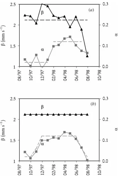
Fig. 10. For the period from September 1997 to August 1998: (a) monthly values of the best fit parameters αand β in Eq. (14); (b) monthly values of the best fit parameterαwithβset to 2.12. Dashed lines show the general trend of each parameter.
Fig. 11. Soil heat flux, G, modelled vs. measured values: (a) period with a fully developed understorey (July–November:α =0.02,
β=2.12 mm s−1;R2=0.89, slope=0.89, intercept=0.34) and (b) with little understorey (December–June:α=0.12,β=2.12 mm s−1; R2=0.94, slope=0.92, intercept=1.25).
It is then possible to calculate the coefficientsαand
β for each month of the year. Their month-to-month variation is represented in Fig. 10a. The coefficient
β is nearly constant throughout the year with mean
β ≈ 2.20 mm s−1, e.g. β−1 ≈ 455 s m−1, except in
July–August 1998 whereβtakes a smaller value than during the preceding months. The reason for this is unclear. In what follows we will consider that β
is constant over the year and equal to 2.12 mm s−1
(mean value including July and August). Such a large value of the resistanceβ−1 (472 s m−1) is caused by the resistance to air diffusion through the litter and the air layer at the soil surface, which is likely to be quite large in this environment with very low wind. However, it is still much lower than a resistance to molecular diffusion through 5 cm of air, that can be estimated about 2300 s m−1, taking 21.5 mm2s−1for
the molecular diffusivity (Campbell, 1977).
The values obtained fora can be grouped in two
categories or periods: from September 1997 to Jan-uary 1998,α≈0.02 and from February to June 1998
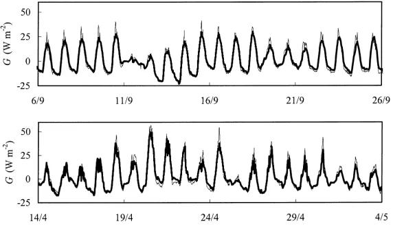
Fig. 12. Evolution of modelled and measured soil heat flux,G, for 20 days in September 1997 (α=0.02,β=2.12 mm s−1) and 20 days
in April 1998 (α=0.12,β=2.12 mm s−1).
to June 1998,αtakes a mean value of 0.12 while it is nearly zero during the other months.
The coefficients α and β do not seem to change with soil water content, whereas we saw in a preced-ing section that the daily amplitude of soil heat flux increases with soil water content. In fact, this is not contradictory because soil water content is likely to influence also the amplitude of the difference between air and litter temperatures.
Fig. 11a and b compare the modelled soil heat flux values for the two periods with experimental values. The agreement is very good for the whole set of data. In particular, the model reproduces well the occa-sional accidents in soil heat flux during periods of cooling or heating, as is visible in Fig. 12 that dis-plays temporal variations of both fluxes in Septem-ber 1997 (with understorey) and April 1998 (without understorey).
A more deterministic model would consist in us-ing a simple two-layer model such as the force-restore model (Deardoff, 1978) along with Eq. (14), with the
Tl,sbeing the ‘surface’ temperature of the force-restore
model. Then, we would need only the air temperature at 20 cm to estimate, at the same time, the soil heat flux and the soil surface temperature. Such a model could be integrated in a multi-layer model with a tur-bulent transfer sub-model that would compute, from air temperature data above the canopy, air temperature profiles above and within the stand. This is the object of current work.
6. Conclusion
In this paper, we presented a method for estimating soil heat flux from temperature, humidity and bulk density profiles. This method is accurate if used with a large set of data and has the advantage of requiring only shallow temperature and humidity probes. Its ac-curacy was confirmed by several tests such as the es-timation of soil thermal conductivity at a given depth or the good closure of the understorey energy budget (Lamaud et al., 2000). It can be used in future programmes devoted to long-term ecological studies. Improvements of the method for such studies could consist in (1) reducing the temperature and humidity profiles to a layer of 10–20 cm, but (2) using more probes for each profile and more profiles on each site, and (3) having a humidity profile for each temperature profile.
This work shows that the amount of heat stored in a forest floor is not negligible over the daily and yearly cycles of the understorey energy budget, and that its estimation is necessary in ecological studies. At our site, this flux represents up to 50% of midday net radiation under the canopy and amounts to 50% of the energy stored between September 1997 and February 1998. Also, the major source of variation of its daily amplitude, when compared to that of transmitted net radiation, is due to soil water content.
surface energy balance could be simplified as G =
αRn,t(t−1t )−Hsoil, whereRn,tis the net radiation
above the understorey, Gthe soil heat flux andHsoil
the sensible heat flux at the soil surface. The latter appears proportional to the difference between soil and air temperatures. The time delay can be taken constant all over the year and equal to 30 min. The ‘soil surface resistance’ can also be considered con-stant throughout the year, and equal to 472 s m−1.
The net radiation term in the surface energy balance equation is small for most of the year, but a bias is introduced if it is neglected between December 1997 and June 1998, e.g. when the understorey was not fully developed. Then, soil heat flux is computed from air temperature and net radiation measurements. The agreement with experimental values is good for the whole data set. Further modelling is in progress to avoid measuring soil temperature.
Acknowledgements
The authors would like to thank Prof. K.T. Paw U for helpful comments during his stay in our laboratory in June–August 1998. We also thank A. Kruszewski for his technical assistance and Dr. D. Arrouays for having provided us with the soil bulk density pro-file. This work was performed during the EUROFLUX project supported by the European Commission under contract ENV4-CT95-0078 (Environment and Climate Programme).
References
Berbigier, P., Bonnefond, J.M., 1995. Measurement and modelling of radiation transmission within a stand of maritime pine (Pinus pinaster Ait.). Ann. Sci. For. 52, 23–42.
Berbigier, P., Bonnefond, J.M., Melmann, P., 2000. CO2and water
vapour fluxes for two years above Euroflux forest site. Agric. For. Meteorol., Submitted for publication.
Campbell, G.S., 1977. An Introduction to Environmental Biophysics. Springer, New York, 159 pp.
Camuffo, D., Bernardi, A., 1982. An observational study of heat fluxes and their relationship with net radiation. Boundary-Layer Meteorol. 23, 359–368.
Cellier, P., Richard, G., Robin, P., 1996. Partition of sensible heat fluxes into bare soil and the atmosphere. Agric. For. Meteorol. 82, 245–265.
Clapp, R.B., Hornberger, G.M., 1978. Empirical equations for soil hydraulic properties. Water Resourc. Res. 14, 601–604. Deardoff, J.W., 1978. Efficient prediction of ground surface
tempe-rature and moisture, with inclusion of a layer of vegetation. J. Geophys. Res. 83 (C4), 1889–1903.
de Vries, D.A., 1963. Thermal properties of soils. In: Van Wijk, W.R. (Ed.), Physics of Plant Environment. North-Holland, Amsterdam, The Netherlands, pp. 210–235.
de Vries, D.A., Philip, J.R., 1986. Soil heat flux, thermal conduc-tivity, and null-alignment method. Soil Sci. Soc. Am. J. 50, 12–18.
Diawara, A., 1990. Echanges d’énergie et de masse à l’intérieur et au-dessus d’une forêt de pins maritimes. Univ. Blaise-Pascal, Clermont-Ferrand II, France, 162 pp.
Idso, S.B., Aase, J.K., Jackson, R.D., 1975. Net radiation-soil heat flux relations as influenced by soil water content variations. Boundary-Layer Meteorol. 9, 113–122.
Kimball, B.A., Jackson, R.D., 1979. Soil heat flux. In: Barfield, B.J., Gerber, J.F. (Eds.), Modification of the aerial environment of crops. Am. Soc. Agric. Eng. 211–229.
Kimball, B.A., Jackson, R.D., 1975. Soil heat flux determination: a null-alignment method. Agric. Meteorol. 15, 1–9.
Kondo, J., Saigusa, N., 1994. Modelling the evaporation from bare soil with a formula for vaporization in the soil pores. Meteorol. Soc. Jpn. 72, 413–420.
Lamaud, E., Ogée, J., Brunet, Y., Berbigier, P., 2000. Validation of eddy flux measurements above the understorey of a pine forest. Agric. For. Meteorol. 106, 189–205.
Lang, A.R., 1987. Simplified estimate of leaf area index from trans-mittance of the sun’s beam. Agric. For. Meteorol. 41, 179–186. Loustau, D., Cochard, H., 1991. Utilisation d’une chambre de transpiration portable pour l’estimation de l’évapotranspiration d’un sous-bois de pin maritime à molinie (Molinia coerulea L. Moench). Ann. Sci. For. 48, 29–45.
McCaughey, J.H., Saxton, W.L., 1988. Energy balance storage terms in a mixed forest. Agric. For. Meteorol. 44, 1–18. Press, W.H., Teukolsky, S.A., Vetterling, W.T., Flannery,