EXTRACTING URBAN MORPHOLOGY FOR ATMOSPHERIC MODELING FROM
MULTISPECTRAL AND SAR SATELLITE IMAGERY
S. Wittke a, K. Karila a, E. Puttonen a, A. Hellsten b, M. Auvinen b,c, M. Karjalainen a
a Finnish Geospatial Research Institute, 02430 Masala, Finland - (firstname.lastname)@nls.fi b Finnish Meteorological Institute, 00101 Helsinki, Finland - [email protected] c Department of Physics, University of Helsinki, Finland – [email protected]
Commission I, WG I/8
KEY WORDS: Urban Morphology, Land Cover Classification, Digital Surface Model, Sentinel-2, TanDEM-X, Satellite Remote Sensing
ABSTRACT:
This paper presents an approach designed to derive an urban morphology map from satellite data while aiming to minimize the cost of data and user interference. The approach will help to provide updates to the current morphological databases around the world. The proposed urban morphology maps consist of two layers: 1) Digital Elevation Model (DEM) and 2) land cover map.
Sentinel-2 data was used to create a land cover map, which was realized through image classification using optical range indices calculated from image data. For the purpose of atmospheric modeling, the most important classes are water and vegetation areas. The rest of the area includes bare soil and built-up areas among others, and they were merged into one class in the end. The classification result was validated with ground truth data collected both from field measurements and aerial imagery. The overall classification accuracy for the three classes is 91%.
TanDEM-X data was processed into two DEMs with different grid sizes using interferometric SAR processing. The resulting DEM has a RMSE of 3.2 meters compared to a high resolution DEM, which was estimated through 20 control points in flat areas. Comparing the derived DEM with the ground truth DEM from airborne LIDAR data, it can be seen that the street canyons, that are of high importance for urban atmospheric modeling are not detectable in the TanDEM-X DEM. However, the derived DEM is suitable for a class of urban atmospheric models.
Based on the numerical modeling needs for regional atmospheric pollutant dispersion studies, the generated files enable the extraction of relevant parametrizations, such as Urban Canopy Parameters (UCP).
1. INTRODUCTION
According to the World Health Organization (WHO, 2016) 98% of low-income and 56% of high income countries do not meet the WHO air quality guideline in urban areas. In cities the sources of particles and hazardous gasses are packed on small areas together with a dense population exposed to health risks due to poor air quality (Ching, 2007). In order to assess the exposure of urban population and predict the dispersion of particles and hazardous emissions, air flow and its interaction with the urban landscape has to be modeled. Urban atmospheric models utilize as input meteorological and geographical information where the latter is typically represented through elevation and land cover datasets. Satellite remote sensing is one tool to provide a constantly updated urban morphology for a broad area. Current mesoscale weather prediction and microscale dispersion models do not perform well in urban areas (Ching, 2007).
Urban morphology derivation by different means has been researched for a while, as the resulting models can be used for a variety of purposes such as for example environmental impact studies, general city planning and atmospheric modeling. Urban morphological models such as BDTopo (Long et al., 2003), NUDAPT (Ching et al., 2009) and WUDAPT (Stewart et al., 2012) all represent the urban morphology in some way derived by different means. While BDTopo and NUDAPT are national databases of France and the U.S. respectively, WUDAPT aims to cover all bigger cities in the world. All have in common that they are not (yet) automated and require either purchased datasets or a professional user to do the processing. This paper
investigates the possibility to derive a minimum of urban morphology represented as a Digital Elevation Model (DEM) and a land cover classification from satellite remote sensing data and a minimal user interference in the processing of those.
The term DEM is an umbrella term for many different ways to mathematically represent the elevation of points in a coordinate system. It is often used to describe the elevation of the bare-earth void of vegetation and manmade structures, which then can also be called for a Digital Terrain Model (DTM). The DEM derived in this work is a Digital Surface Model (DSM) representing the elevation on top of reflective surfaces, meaning manmade structures and vegetation is included. (Maune et al., 2001)
2. DATA AND METHODS
This paper combines the techniques of optical and radar remote sensing to obtain morphological information of the urban environment. The goal was to design as automatic process as possible and that the process would be applicable to cover large areas with minimal production costs. Currently, there are satellite missions that provide free data globally, e.g., ESAs Sentinel-2 and NASAs Landsat-8 missions. We decided to use Sentinel-2 images in this project to make use of the higher resolution of the images. For the DEM creation we used the German TanDEM-X data, which is not free, but provides global data set and can be used at no cost for scientific purposes.
2.1 Area of Investigation
The test area is located in southern Finland and covers the metropolitan area of Helsinki, including Helsinki, Espoo and parts of Vantaa and covers an area of approximately 39 x 27 kilometers (cf. Figure 1)
.
Figure 1: Area of investigation defined by the corner coordinates 6021’30’’N, 2502’21’’E and 6006’30’’N, 2428’21’’E with subareas of Helsinki and Espoo (green) and downtown Helsinki (turquoise)
2.2 Land Cover Classification
2.2.1 Sentinel-2 is one of the satellite missions of the Copernicus program which was officially initiated in 2008 by the European Commission. The space segment of the program consists of seven satellites whereof Sentinel-2 is responsible for high resolution optical data for land services. (Hoesch, 2015)
Table 1: Sentinel-2 central wavelengths and resolution of the 13 bands (after ESA, 2017b)
Bands
central wavelength
[nm]
resolution [m]
Band 1 – coastal aerosol 443 60
Band 2 – blue 490 10
Band 3 – green 560 10
Band 4 – red 665 10
Band 5 –veg. ‘red edge’ 705 20
Band 6 –veg. ‘red edge’ 740 20
Band 7 –veg. ‘red edge’ 783 20
Band 8 – NIR 842 10
Band 8A – veg. ‘red edge’ 865 20
Band 9 – water vapor 945 60
Band 10 – cirrus 375 60
Band 11 – SWIR 1610 20
Band 12 - SWIR 2190 20
Sentinel-2 follows among others the successful missions of the Landsat program of the United States (NASA, 2017) and the French SPOT satellite systems (CNES, 2017) and gives an update in terms of resolution, data availability and number of bands.
We used one Sentinel-2 image that was totally cloud free in the area of investigation, acquired on 17. August 2015 obtained as level-1C product from ESAs Sentinel-2 data hub. This product is radiometrically and geometrically corrected, including ortho-rectification and spatial registration on a global reference system. After downloading, a subset of the image was created
using SNAP toolbox (ESA, 2017) subset-tool. The level 1C provides top-of-atmosphere data, which means that disturbances due to aerosols in the air between sensor and Earth's surface are still present in the product. With sen2cor ESA provides a processor to do the atmospheric, terrain and cirrus correction that then delivers a corrected reflectance image to the user which is also called level 2A product. (Hoesch, 2015)
2.2.2 Land Cover Classification. The purpose of image classification procedures of multispectral images is the automatic categorization of all image pixels into land cover classes or themes based on the spectral reflectance in different wavelength intervals. The land cover classification can be utilized in urban atmospheric models to assign different surface types, for example, predefined roughness factors or forest canopy parametrizations, which strongly influence the flow dynamics near the ground level.
Besides supervised and unsupervised classification approaches, the determination of specific classes based on their reflectance behavior in class specific wavelength intervals can be used. Besides using only one band thresholding, indices have been widely used (e.g. Dong et al. (2015) and Du et al. (2016)).
Vegetated areas can for example be identified using the Normalized Difference Vegetation Index (NDVI):
NDVI = (NIR – red) / (NIR + red) (1)
This Index was first used by Rouse et al. (1973) for determining the general fitness of vegetation, but it can also be used to distinguish vegetation covered from not vegetated areas such as built-up areas. The vegetated areas can then be distinguished by setting a threshold value manually or using an automatic thresholding algorithm like for example the one introduced by Otsu (1975). The NDVI is normalized by default to the range -1 to 1, which also allows the comparison of images that have been acquired under different conditions.
Water areas are another class that can be distinguished by using an index. McFeeters (1996) suggested the use of a water index, similar to known vegetation indices. Equation 2 shows the formula for obtaining the Normalized Difference Water Index (NDWI). In 2007, Xu et al. suggested an extension to the NDWI by using shortwave/middlewave infrared band (in our case band 11) instead of near infrared to remove built-up land noise in the water index image. It is called the modified NDWI (mNDWI), shown in Equation 3. As the study area contains a lot of built-up area we used the mNDWI index.
NDWI = (green – NIR) / (green + NIR) (2)
mNDWI = (green – SWIR) / (green + SWIR) (3)
Regarding the band designations of Sentinel-2 (cf. Table 1) it can be seen that the green band 3, as well as the NIR band 8 have a resolution of 10 meter, whereas the SWIR band 11 has a resolution of 20 meter. Du et al. (2016) describes a method to deal with that problem without losing the higher detail of the RGB and NIR bands by using the 10 meter resolution bands to upscale the SWIR band to 10 meter based on pan-sharpening algorithms. In our case however, the additional uncertainties that are associated with the new assumptions made for the pan-sharpening are not desired. Disregarding the different sizes of a resolution cell of the SWIR and green band will only result in the equation considering four smaller cells with the same SWIR
value as the bigger one. For the extraction of built-up areas the NDBI has been used in different variations (e.g. Xu, 2007 and Zha et al., 2003).
The combination of above mentioned Indices results in three classes: vegetation, water and ‘other’. The ‘other’ class consisting of everything that is not being recognized as water or vegetation, like for example dead, non-green or unhealthy vegetation, built-up area, sand and rock.
2.2.3 Accuracy Assessment. A standard way of representing the accuracy of the land cover classification is an error matrix, where the classification result is compared to ground truth reference data (Congalton, 1991). Reference data has been collected in the time from 6th to 15th September 2016 on 6 field survey campaigns. A systematic sampling method was chosen with two areas of investigation. First, the downtown area in vegetation, building, street and water. Building and street classes were combined later to fit to the 3 class classification through the indices. With this dataset the error matrix and value were calculated.
2.3 Digital Elevation Model
2.3.1 The TanDEM-X (TerraSAR-X add on for Digital Elevation Measurement) mission is a public private partnership of EADS Astrium GmbH and the German Aerospace Center (DLR). Launched in June 2010, TanDEM-X is an addition to the identically constructed TerraSAR-X satellite operating in orbit since 2007, which together form the first configurable SAR interferometer in space. Both satellites are flying in helix formation, which gives the opportunity to perform along track, as well as across track interferometry. The primary mission goal of the formation is the generation of the global WorldDEM product with 12 meter raster size and a vertical accuracy of better than 2 meter. As the first of its kind, the mission is also used to test new techniques of SAR-interferometry to find new possible applications. The X in the names of both satellites corresponds to X-band RADAR which shows the operating interval of the wavelength around 3 cm at the center frequency of 9.65 GHz aimed at providing a high interferometric sensitivity.
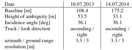
The TanDEM-X scenes used in this paper are from 16.07.2013 and 14.07.2014 with an effective baseline of 108.36 and 175.15 meters, respectively, both ascending and right looking (cf. Table 2). The received images were provided in CoSSC (Coregistered Single look Slant range Complex).
Table 2: Properties of the used TanDEM-X bistatic image pairs
Date 16.07.2013 14.07.2014
Baseline [m] 108.4 175.2
Height of ambiguity [m] 53.5 33.1
Incidence angle [deg] 36.1 36.1
Track / look direction ascending / right
2.3.2 DEM-Generation. To generate a DEM, two SAR images are used. Those images must have an appropriate geometric baseline (typically in order of tens or hundreds meter) to form an interferometric pair. In case of TanDEM-X the two images are acquired simultaneously. As mentioned, TerraSAR-X and TanDEM-X satellites fly in helix formation for exactly this purpose. Given the non-existing temporal baseline, temporal decorrelation is not a problem. That means that there is no change on earth surface in terms of microwave radiation between the acquisitions and the atmospheric conditions for the simultaneous acquisitions are the same. However, volumetric decorrelation in vegetated areas still exists. (Massonnet et al., 1998)
The interferogram is generated through the phase difference of two SAR images, master (TanDEM-X) and slave (TerraSAR-X) image.
The main steps for DEM generation are the following:
1. Flattened interferogram generation
2. Multilooking, phase filtering and coherence estimation
3. Phase unwrapping
4. Absolute phase calibration and phase to height conversion
5. Geocoding (Wessel et al., 2013)
The process is nearly automatic. As INSAR is a relative measurement method, the interferometric DEM always needs a reference height from the user. This can be provided as an external DEM, ground control points or one single reference height of the point in the center of the processed scene, which is then used to derive a height model (at this point user interference is always necessary). According to Kim et al. (2011) and Chunxia et al. (2012) it is better to use an external DEM for height reference as this is the most accurate way.
In the selection of interferometric data there is always a tradeoff in choosing between the better accuracy but more complicated and error-prone phase unwrapping of longer baselines and higher error allowing but better phase unwrapping of shorter baselines. In this study two DEMs have been created. A DEM with a shorter effective baseline and coarser spatial resolution (10 meter) was used as a reference DEM for the finer DEM (5 meter spatial resolution).
2.3.3 Accuracy Assessment. The accuracy of a DEM is a measure of how good the modeled elevation of a grid cell approaches the true surface value in the same point or area. This accuracy is measured in both horizontal and vertical axes. Earlier, the horizontal accuracy for the TerraSAR-X mission has been evaluated for example by Ager and Bresnahan (2009), who estimated the horizontal accuracy to be about 1 meter on average. This also accounts for the TanDEM-X mission.
The quality of the input data, the DEM resolution and data
We used freely available airborne laserscanning data provided by NLS (NLS, 2017) as ground truth DEM. It was downloaded and converted into a similar DEM with a raster size of 5 m. In order not to get a wrong impression of accuracy that is depending on the different resolutions of the two datasets, 20 open areas without any objects have been selected as control points, such as soccer fields and parking lots.
The RMSE requires a normal distribution of errors and that all systematic errors have been removed (Daniel et al., 2001). For the present dataset the normal distribution is assumed and the systematic error is estimated by the average difference between the two DEMs. This error is then subtracted from the DEM to be assessed.
To evaluate the spatial distribution of the error, another approach was been chosen to help understanding the strengths and weaknesses of the InSAR-DEM. QGIS raster calculator was used to subtract the ALS-DEM values cell by cell from the InSAR-DEM to generate a difference grid of 5 by 5 meter.
3. RESULTS AND DISCUSSION
3.1 Land Cover Classification
Figure 2 shows the result of the use of indices. It shows the water and vegetated areas as classified through the use of the NDVI and MNDWI and further user supervised thresholding at 0.6 and 0.5 respectively after visual inspection.
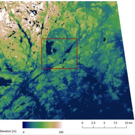
Figure 2: Resulting water and vegetation areas (white areas show class ‘other’) from indices of the whole test site, extracted from Sentinel-2 image from 17.08.2015. Red square indicates location of Figure 3.
The accuracy assessment of the classification was done using the error matrix. The matrix can be seen in Table 3. The matrix also provides the omission and commission errors for each class, which provide a more detailed description of distribution of the error among the classes. The overall accuracy of the classification was calculated to be 91%, and 0.81 for �.
Classification accuracy was found to be sufficient for the evaluation purpose (personal communication FMI, 2017). The indices MNDWI and NDVI were used to identify water and
vegetated areas. This leaves a third class, named 'other'. This class includes open soil, bare rock, urban structures as well as water and vegetated areas that were not identified as those.
Table 3: Error matrix for accuracy assessment of the land cover classification
Figure 3 also shows that most of the shore areas and small rivers that are in the map are not covered by the water mask. This is due to the different spectral response of shallow water areas or vegetation or other objects covering the water during image acquisition. Also the presence of algae in the water can influence the spectral response. The smaller rivers and streams in the map are not covered, because the width of the river does not cover enough of the 10 by 10 meter pixel of the Sentinel image. With that the water response is not strong enough and cannot be identified as water. It should be noted that even though the topographic map is the most actual, it might not show today's extent of the water areas. In general the transition between water and bordering surfaces can be rather fuzzy than a strict line (Dewi et al., 2016).
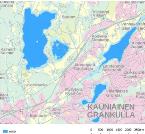
Figure 3: Water areas in the north western part (center coordinate: 6014’47’’N, 2442’32’’E) of the test area, marked by red square in Figure 2, from mNDWI with topographic background map from NLS (2017)
A known problem in image classification is the presence of mixed pixels. Those pixels are for example such that cover the borders of forests to built-up area or the shorelines of lakes where there is still water, but also vegetation present. Those mixed pixels are assigned to the class that is covering most of the area of the pixel, which can be difficult to assign in field work. Therefore the location of the erroneous pixels has been checked by coloring the sample points according to their agreement with the observed ground truth.
As the classification is based on an image taken in summer 2015 and the field survey was done in summer 2016 the extent of the water and vegetated areas might differ. Also the vegetation classification is dependent on the fitness and water content of the plants (Lillesand et al., 2008), which cannot easily be determined in the field.
3.2 DEM
Figure 4 shows the resulting raw DEM with a grid spacing of 5 meter, as it was produced following the DEM-generation methodology. It can be seen that there are random artifacts in the water and land areas and no-data holes in land areas.
Figure 5 shows the same DEM after application of the water mask from the Sentinel-2 image, the interpolation of the no data cells in land areas and the removal of the systematic error of 16.5 meters.
Figure 4: Raw DEM of the whole test area after DEM processing steps, black indicates no data
The RMSE of the check points was found to be 3.2 meter. As an example of the spatial distribution of the difference in dense urban area between the two DEMs, the area around Hotel Torni in downtown Helsinki is shown in Figure 6. Hotel Torni was chosen to be the center of higher level investigation, as it is a 69.5 meter high landmark in the city center of Helsinki which also functions as an urban meteorological measurement station.
As shown in Figure 4, the first raw DEM had holes and artefacts which arise due to different reasons. One is low coherence in densely built-up areas from the shadows of the buildings that are imaged in a side-looking geometry. Low coherence in general can come from moving objects or surface materials, that results in a low backscatter. On land areas, artefacts may arise from geometrical distortion and low backscatter due to the roof surface material of the buildings. (Martone et al., 2013) Another influencing factor is the orientation of the building in relation to the aspect angle of the SAR antenna (Henderson et al., 1998).
Figure 5: Final DEM of the whole test area after post processing, red square indicates location of Figure 3
The water areas extracted from the Sentinel-2 image solve the problem of artefacts in the water areas by masking them out. However, shore areas and water areas that do not cover a whole Sentinel-2 resolution cell are not covered consistently. This comes due to the fact that the water areas are determined through the green and SWIR channel, which have a resolution of 10 and 20 meter. Water areas often have a shallow transition to land areas, where the reflectance is not only water but also the ground or if present, vegetation.
Figure 6: Difference between TanDEM-X derived DEM and ALS DEM represented as 5 by 5 meter grid in the area around Hotel Torni (green circle), Helsinki (center coordinate: 6010’03’’N, 2456’18’’E)
The use of the elevation model in urban atmospheric modeling requires a certain degree of urban structure representation. The first shortcoming of the TanDEM-X InSAR processing is the 5 meter resolution. In that way only structures bigger than 5 by 5 meter are covered. Another restriction comes from the image difference in detail between the TanDEM-X DEM and the ALS DEM arises due to the different resolution of the original data and the interferometric processing. Due to the presence of noise (speckle) in SAR images, they need to be filtered, which smoothens the DEM. In addition, continuity is assumed during phase unwrapping, it cannot adapt to abrupt changes in height. Therefore and due to the interpolation of the no data areas, the TanDEM-X DEM is much smoother than the ALS DEM. Areas, where the ALS DEM shows a significantly higher elevation than the TanDEM-X DEM (orange in Figure 6) seem to be cells in border areas of buildings or whole buildings that are missing in the TanDEM-X DEM. Missing buildings in the TanDEM-X DEM can occur due to the time difference between the acquisition of the raw data used for generation of both DEMs. Another reason could be a strong double bounce scattering from the ground and building wall. This could result in dislocated ground heights.
3. CONCLUSION
This work presents the design and derivation of urban morphology map based on free or low-cost remote sensing data, with the aim to optimize the automation of the urban morphology derivation process. The user requirement was a digital elevation model as well as a land cover classification with at least three classes (water, vegetation, 'other'). Based on the outcomes of the work presented here, it can be concluded that all requested features could be produced.
The two files created have to be considered separately, as they use very different raw data that both need a special processing workflow.
First, the DEM was successfully produced from TanDEM-X data in a 5 meter grid with a vertical accuracy of ~3.2 m. After InSAR processing, the initial model was improved by interpolation and the use of a water mask produced from the Sentinel-2 image. For urban areas especially the DEM lacks important information on buildings and street canyons, which can only be improved by the use of ancillary data or more urban structures like buildings and streets as well as water and vegetated areas that were not classified as those. The classification was done by using two normalized difference indices, namely the NDVI and MNDWI and user supervised thresholding. The grid size of the resulting classification is 10 times 10 meters, which was selected to correspond the pixel size of the used Sentinel-2 bands. The classification accuracy was approved to be sufficient for urban atmospheric modeling with neighborhood- scale resolution where the relevant flow phenomena are larger than the individual buildings (Tack et al., 2012).
The results show that it is possible to create a sufficient morphological database for urban atmospheric modeling at neighborhood-scale resolution. The use of the database in other fields, such as for example flood modeling is not advisable due to its limitations in modeling the ground between the surface features and the omission of other surface features, such as orientation and material.
We are aware that also the classification could be improved by the use of ALS data to distinguish between higher and lower single trees and other small patches of vegetation do not affect the airflow as much as they do in urban areas. Also as mentioned earlier, ALS data is expensive to acquire and covers only a small area in a certain time frame.
Extensions of the presented morphological database can make it possible to use it in other fields as well, such as flood modeling or traffic pollution modeling. These extensions can for example be streets or building footprints from open sources like Openstreetmap (http://www.openstreetmap.org). Another way would be to make use of the newly formed data portals of cities providing free geospatial data like Hamburg (http://transparenz.hamburg.de) or Helsinki (http://kartta.hel.fi/avoindata/).
A further step to assess the performance of the urban morphological database in atmospheric modeling would be to use it as morphological input for urban atmospheric models. Also it will be investigated, to what extent it is possible to derive the urban canopy parameters (UCP) from this database, similar to the UCP derivation done from ALS data in Burian et al. (2004).
ACKNOWLEDGEMENTS
The authors would like to acknowledge the financial support from Academy of Finland research projects ‘Urban Morphology and Atmospheric Boundary Layer Modeling’ (CityClim: decision number 277734) and ‘Integration of Large Multisource Point Cloud and Image Datasets for Adaptive Map Updating ‘ (295047).
REFERENCES
Burian, S. J., Stetson, S. W., Han W., Ching J., Byun, D., 2004. High resolution dataset of urban canopy parameters for Houston, Texas. In: Proceedings of the Fifth Symposium on the Urban Environment, American Meteorological Society, Vancouver, BC.
Ching, J., 2007. National Urban Database and Access Portal Tool, a project overview. In: Proceedings of the Symposium on Urban Environment 7.
Ching, J., Brown, M., McPherson, T., Burian, S., Chen, F., 2009. National Urban Database and Access Portal Tool. In: Bulletin of the American Meteorological Society 90.8, pp. 1157–1168.
CNES, 2017. Spot – Earth seen from space. https://spot.cnes.fr/en/SPOT/index.htm (10.04.2017)
Congalton, R.G., 1991. A review of accessing the accuracy of classifications of remotely sensed data. In: Remote Sensing of the Environment, 37, pp. 35-46.
Dewi, R.S., Bijker, W., Stein, A., Marfai, M.A., 2016. Fuzzy Classification for Shoreline Change Monitoring in a Part of the Northern Coastal Area of Java, Indonesia. In: Remote Sensing 8.3, p. 190.
Dong, T., Meng, J., Shang, J., Liu, J., Wu, B., 2015. Evaluation of Chlorophyll-Related Vegetation Indices Using Simulated Sentinel-2 Data for Estimation of Crop Fraction of Absorbed Photosynthetically Active Radiation. In: IEEE Journal of Selected Topics in Applied Earth Observations and Remote Sensing 8.8, pp. 4049–4059.
Du, Y., Zhang, Y., Ling, F., Wang, Q., Li, W., 2016. Water Bodies’ Mapping from Sentinel-2 Imagery with Modified Normalized Difference Water Index at 10 m Spatial Resolution Produced by Sharpening the SWIR Band. In: Remote Sensing 8.4, p. 354.
ESA, 2017. STEP – Science toolbox exploitation platform. http://step.esa.int/main/toolboxes/snap/ (10.04.2017)
ESA, 2017b. Sentinel-2 Spatial Resolution. https://earth.esa.int/web/sentinel/user-guides/sentinel-2-msi/resolutions/spatial (10.04.2017)
Henderson, F.M., Lewis, A.J., 1998. Principles & Applications of Imaging Radar – Manual of Remote Sensing. Ed. by F.M. Henderson, A.J. Lewis. American Society for Photogrammetry and Remote Sensing.
Hoesch, B., 2015. Sentinel-2 User Handbook. Ed. by B. Hoesch. ESA Standard Document.
Kim, N., Bijker, W., Tolpekin, V.A., 2011. 2.5D building Reconstruction from SAR and Optical Data Using OOA.
Lillesand, T. M., Kiefer, R. W., Chipman, J. W., 2008. Remote sensing and image interpretation. Hoboken (N.J.): John Wiley & Sons.
Long, N., Mestayer, P. G., Kergomard, C., 2003. Urban Database Analysis for mapping morphology and aerodynamic parameters: the case of St. Jerome sub-urban area, in Marseille
during ESCOMPTE. In: Improved Models for computing the roughness parameters of urban areas: D4.4 FUMAPEX report. Ed. by A. Baklanov, S. Joffre.
Martone, M., Rizzoli, P., Bräutigam, B., Krieger, G., 2013. First 2 years of TanDEM-X mission: Interferometric performance overview. In: Radio Science 48.5, pp. 617–627.
Massonnet, D., Feigl, K.L., 1998. Radar interferometry and its application to changes in the Earth’s surface. In: Reviews of Geophysics 36.4, pp. 441–500.
Maune, D. F., Blake, T.A., Constance, E.W., 2001. Digital elevation model technologies and applications: the DEM users manual. Ed. by D. F. Maune. Bethesda, MD: American Society for Photogrammetry and Remote Sensing. Chap. DEM User Requirements, pp. 441–460.
McFeeters, S.K., 1996. The Use of the Normalized Difference Water Index (NDWI) in the delineation of open water features. In: International Journal of Remote Sensing 17.
NASA, 2017. Landsat Missions. https://landsat.gsfc.nasa.gov/ (10.04.2017)
NLS, 2017. NLS file service of open data. https://tiedostopalvelu.maanmittauslaitos.fi/tp/kartta?lang=en (10.04.2017)
Otsu, N. A, 1975. Threshold selection method from Gray-Level histograms. In: IEEE T. Syst. Man. Cyb. 9, 62–66.
Rouse, J.W., Haas, R.H., Schell, J.A., Deering, D.W., 1973. Monitoring vegetation systems in the Great Plains with ERTS. In: Proceedings of the Third ERTS Symposium, pp. 309 –317.
Stewart, I. D., Oke, T. R., 2012. Local Climate Zones for Urban Temperature Studies. In: Bulletin of the American Meteorological Society 93.12, pp. 1879–1900.
Tack, A., Koskinen, J., Hellsten, A., Sievinen, P., Esau, I., Praks, J., Kukkonen, J. and Hallikainen, M., 2012. Morphology database of Paris for atmospheric modelling purposes. In: IEEE Journal of Selected Topics in Applied Earth Observations and Remote Sensing. 5 (6) pp. 1803-1810.
Wessel, B., 2013. TanDEM- X Ground Segment DEM Products Specification Document. Tech. rep. Deutsches Zentrum für Luft- und Raumfahrt.
WHO, 2016. WHO Global Urban Ambient Air Pollution Database.
http://www.who.int/phe/health_topics/outdoorair/databases/AA P_database_summary_results_2016_v02.pdf?ua=1 (20.12.2016)
Xu, H., 2007. Extraction of Urban Built-up Land Features from Landsat Imagery Using a Thematic Oriented Index Combination Technique. In: Photogrammetric Engineering & Remote Sensing 73, 1381–1391.
Zha, Y., Gao, J., Ni, S., 2003. Use of normalized difference built-up index in automatically mapping urban areas from TM imagery. In: International Journal of Remote Sensing 24.3, pp. 583–594.