GLOBAL CHANGES IN THE SEA ICE COVER AND ASSOCIATED SURFACE
TEMPERATURE CHANGES
Josefino C. Comiso
Cryosphere Sciences Laboratory, NASA Goddard Space Flight Center, Greenbelt, MD, USA 20771
Comission VIII, WG VIII/6 Chair, Invited Paper, ID 2114
KEYWORDS: Global, sea ice, surface temperature, trends, climate change, remote sensing
ABSTRACT
The trends in the sea ice cover in the two hemispheres have been observed to be asymmetric with the rate of change in the Arctic being negative at -3.8% per decade while that of the Antarctic is positive at 1.7% per decade. These observations are confirmed in this study through analyses of a more robust data set that has been enhanced for better consistency and updated for improved statistics. With reports of anthropogenic global warming such phenomenon appears physically counter intuitive but trend studies of surface temperature over the same time period show the occurrence of a similar asymmetry. Satellite surface temperature data show that while global warming is strong and dominant in the Arctic, it is relatively minor in the Antarctic with the trends in sea ice covered areas and surrounding ice free regions observed to be even negative. A strong correlation of ice extent with surface temperature is observed, especially during the growth season, and the observed trends in the sea ice cover are coherent with the trends in surface temperature. The trend of global averages of the ice cover is negative but modest and is consistent and compatible with the positive but modest trend in global surface temperature. A continuation of the trend would mean the disappearance of summer ice by the end of the century but modelling projections indicate that the summer ice could be salvaged if anthropogenic greenhouse gases in the atmosphere are kept constant at the current level.
1. INTRODUCTION
Sea ice has been regarded as a key component of the Earth’s climate system. It covers about 6% of the World’s oceans and affects the system in many ways. For example, sea ice keeps ocean heat from being released to the atmosphere in winter while it limits the amount of heat from the sun that is absorbed by the ocean in summer. Sea ice also causes the redistribution of salt in the ocean because salinity is enhanced through brine rejection where it forms while salinity is reduced where it melts in the spring and summer. The melt of sea ice in spring and summer has also been associated with the occurrences of ice edge blooms and high productivity near the ice edge regions because the layer of low-density melt water is exposed to abundant sunlight and becomes an ideal platform for photosynthesis (Smith and Comiso, 2008). Moreover, the marginal sea ice region is regarded as the site of strong ocean– atmosphere interactions and is usually visited by intense storm activities known as polar lows, and cold-air outbreaks (Comiso, 2010). Also, the growth of ice in coastal polynyas and other regions causes the production of high salinity and high density cold water that sinks to the bottom and becomes part of the global ocean thermohaline circulation (Gordon and Comiso, 1988). Moreover, changes in the sea ice cover could cause profound effects on the global heat balance and hence the weather and the climate (Fletcher and Kelley 1978).
The advent of satellite observation systems has enabled the compilation of comprehensive and consistent global sea ice cover data from 1978 to the present. Results from analysis of the data have indeed revealed that large changes are going on in the sea ice cover (Comiso et al., 2008; Comiso and Hall, 2014). In the Arctic the yearly averages of the ice extent has been declining at a rate of about 4% per decade while in the Antarctic the ice extent has been increasing at a rate of about 2% per decade. A most visible signal, however, is the observation of a
rapid decline of about 11% per decade of the perennial ice cover in the Arctic. Such decline has been a concern because the perennial ice (or ice that survives the summer melt) in the Arctic has been around and observed in situ for at least 1450 years (Kinnard et al., 2011). The loss of the coverage of the perennial ice has caused a general warming of the region, mainly through ice-albedo feedback, that in turn has led in part to the thawing of the permafrost, melt of glaciers, retreat of snow covered areas, the loss of mass of the Greenland ice sheet, and the greening of the Arctic (Comiso and Hall, 2014; Bhatt et al., 2013; Luthche et al., 2006; Zwally et al., 2002). Since the continuation of the loss of all these various components of the cryosphere could lead to more serious if not irreversible consequences it is critical that more research is done on the variability of the sea ice cover and related variables. It is also important to look at these changes from a global perspective since the trend in the ice cover in the Antarctic is going the opposite ways (Cavalieri et al., 1997). Such asymmetry has been postulated to be caused by various factors including the increase in snow precipitation in the Antarctic, the freshening of water in the region due to increases in the melt of ice shelves (Jacobs, 2006) and the occurrence of the ozone hole that tended to cause a deepening of the lows in the West Antarctic region (Turner et al., 2009). In this study, changes in the sea ice cover, using a sea ice data set that has been enhanced for better consistency and updated for improved statistics, has been evaluated in conjunction with observed changes in surface temperature to gain insight into the phenomenon and improved understanding of the state and future of the sea ice cover.
2. SATELLITE DATA AND QUALITY ASSESSMENT
The observation of the seasonal and interannual variability of the sea ice cover was made possible through the use of data from a series of passive microwave sensors that started with the NASA/Nimbus-7 SMMR. The distribution of the sea ice cover
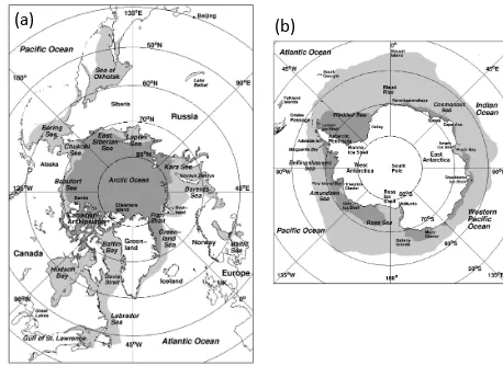
in the two hemispheres are different primarily because of geographical differences. In the Arctic, the sea ice cover is located mainly in the Arctic Ocean basin which is surrounded by land while in the Antarctic, the sea ice cover surrounds a continent called Antarctica. The atmospheric circulation patterns are also different and influenced mainly by the Northern Annular Mode (NAM) in the Arctic and the Southern Annular Mode (SAM) in the Antarctic. The typical distribution of the sea ice cover in the two hemispheres during winter (light gray) and summer (dark gray) are shown in Figures 1a for the Arctic and 1b for the Antarctic. In the Arctic basin the advance of sea ice in winter is restricted by land boundaries but in the peripheral seas the ice goes as far south as 44ºN. In the Antarctic, there is no land boundary and sea ice can go as far north as allowed by surface temperature, ocean current and wind circulation but seldom beyond 55ºS.
Figure 1. Sea ice cover in winter and summer in (a) the Arctic and (b) the Antarctic.
The basic data derived from the passive microwave sensors is sea ice concentration defined as the fraction of ice within the footprint of the sensor. Several algorithms have been developed to derive this parameter at accuracies varying from 5% to 25% depending on season and surface condition (e.g., Cavalieri et al., 1984; Svendsen et al., 1986; Swift et al., 1986; Comiso, 1986; Steffen et al., 1992; Marcus and Cavalieri, 1998). The two that have been most frequently used for time series studies are the NASA Nimbus-7 Team Algorithm (NT1) (Cavalieri et al., 1984) and the Bootstrap Algorithm (Comiso, 1986). An improved version of the NT1 was developed and called NT2 (Markus and Cavalieri, 1998) but is not usually used for the time series studies because it uses an 89 GHz channel which is available continuously only starting in 1992. The Bootstrap Algorithm also underwent some enhancements primarily with the introduction of dynamic tie points for 100% sea ice and 100% open water that better account for daily fluctuations in weather and surface temperature. Ice concentration data have been used to estimate two basic parameters that have been used to quantify the variability and trends in the sea ice cover, namely, ice extent and actual ice area. Ice extent is defined as the integral sum of all areas with ice cover of at least 15% ice concentration while ice area is the area that is actually covered by sea ice and is the sum of the product of the area of each pixel and the concentration of the same pixel in the ice covered regions.
Validation of ice concentration products have been done by a number of investigators and the error in winter has been typically between 5 to 10% while in the summer the error is
usually between 10 to 25%. The larger error in the summer is caused mainly by changes in the changing characteristics of the snow surface and the presence of meltponding that makes the signature of ice covered surfaces difficult to interpret. Another problem is the presence of new ice the signature of which is usually between that of open water and the thicker ice types which dominates the ice cover.
Figure 2. Sea ice cover data over the Sea of Okhotsk using (a) Landsat image on 11 February 2003 and corresponding ice concentration maps from (b) AMSR-E just the 6.25 km high resolution 89 GHz data; (c) AMSR-E using the standard data product generated at 12.5 km resolution; and (d) SSM/I using the historical time series grid at 25 km.
An accepted representation of the true spatial distribution of the sea ice cover during cloud free condition is Landsat data an example of which is shown in Figure 2a. The image depicts the typical distribution of the sea ice cover in the Okhotsk Sea during the middle of winter. The ice cover in the image is shown to consist of components that represent different stages in the growth of sea ice. This includes large ice floes, smaller or broken up ice floes, new ice and ice bands at the ice edge region (right side). To demonstrate that the passive microwave data provides a good representation of the sea ice cover Figures 2b, 2c and 2d show passive microwave images of the same region at the various resolutions they are being generated from AMSR_E data. Figure 2b show ice concentration derived from 89 GHz (H and V) only which provides the best resolution and is mapped at 6.5 km grid. This image illustrates that at high enough resolution passive microwave data is able to capture some details of key features of the ice cover like the divergence area in the middle of the image. Such features are also apparent in Figure 2c which is produced at 12.5 km grid, the standard grid for AMSR-E products, but some of the details captured in Figure 2b are no longer apparent. More of the details are lost in Figure 2d which makes use of the 25 km grid that has been the grid used in historical data set for sea ice. Although much of the details are lost, the 25 km grid data actually provide the best
(a)$ (b)$
quantitative agreement with Landesat data. This is in part because the co-registration of each data element at the lower resolution is not as critical as that at the higher resolution when comparative analysis is made.
For time series studies, it is important to note that the data is made up of measurements from different sensors launched one after another to ensure continuity of the coverage. The different sensors need to have compatible calibration and consistent reference brightness temperatures for 100% sea ice and open water to ensure that the derived geophysical parameters from the different sensors are consistent. The SMMR sensor was followed by a series of the DMSP/SSM/I sensors and also the EOS/Aqua/AMSR-E and the GCOM-W/AMSR2 systems. Monthly data from the sensors that are currently used for sea ice variability studies are presented in Figure 3. The AMSR-E and AMSR2 have provided the most useful and consistent characterization of the sea ice cover so far and mainly through the relatively high resolution information they provide. At the same time it has been problematic to incorporate the data as part of the historical passive microwave time series because of biases associated with the much better resolution of these sensors than the other ones (Comiso and Nishio, 2008). The coarse resolution of SSM/I leads to a less defined (smeared) marginal ice zone that in effect causes the 15% ice edge to be farther away from the pack by as much as almost one pixel (about 25 km) than that of AMSR-E (Comiso and Nishio, 2008). Although the values are generally in agreement, Figure 3 shows that AMSR-E and AMSR2 ice extents are consistently lower than those of SSM/I. There is also a gap in coverage of almost a year between AMSR-E and AMSR2 data. For consistency and to avoid biases that might affect the trend analysis results the time series data used in this study make use of only SMMR and SMM/I data
Figure 3. Monthly ice extents in the Northern Hemisphere as derived from SMMR (in green), SSM/I (in red), AMSR-E (in
blue) and AMSR2 (in purple) sensors.
Surface temperature is likely the most important parameter that is associated with the changing sea ice cover. The extremely harsh and severe weather conditions in the polar regions have made it difficult to obtain comprehensive in situ data in the region. The alternative had been to use reanalysis data (NCEP or ECMWF) but in the polar regions such data are not so reliable because of very limited in situ data which are used as input for the reanalysis models. The most practical way to get good spatial and temporal coverage is to use satellite data and in particular thermal infrared sensor data such as those from the NOAA/Advanced Very High Resolution Radiometer (AVHRR) data. The record length of this data set is about the same as that for passive microwave data but continuous digital data became available only starting August 1981. The data set again consist
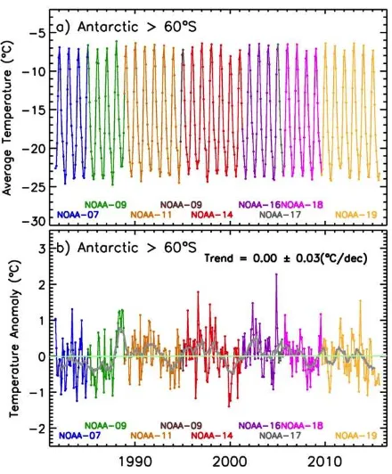
of those from several sensors launched one after another as illustrated in Figure 4. In Figure 4, the monthly average surface temperature for each month from August 1981 to June 2016 are presented with the different colors corresponding to data from the different NOAA/AVHRR sensors. There has been problems of inconsistency in calibration as well as degradation that is aggravated by a slightly changing orbital parameters. Also, surface measurements can only be made during clear skies conditions and the available channels are not ideal for establishing high confidence in the cloud mask. To overcome this problem some techniques were developed to complement the regular cloud mask. Also, in situ data from meteorological stations were used take into account the lack of consistency in the instrument calibration and other problems as described in Comiso (2003). Generally, the resulting data set agrees well with WMO station data and even better with aircraft infrared data (i.e., from Operation Ice Bridge (OIB) project) that has been collected in both Arctic and Antarctic regions.
Figure 4. (a) Monthly averages and (b) monthly anomalies of surface temperature in the Antarctic for the region > 60oS.
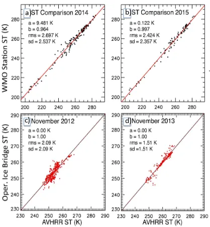
Some examples of such comparative analysis of in-situ or aircraft data with satellite data are shown in Figure 5. The scatter plots in Figures 5a and 5b shows comparisons with data from WMO stations and indicates rms accuracies of 2.7 K and 2.4 for 2014 and 2015 data, respectively. This is a typical result from error analysis of the data done in previous studies (Steffen et al., 1992; Wang and Key, 2003, Comiso, 2003). The uncertainties in the plots, however, may not be due to uncertainties in the satellite measurements alone since the in situ measurements also have some uncertainty issues. Thermal infrared aircraft data from the operation ice bridge project actually compared better and yielded improved accuracies with rms error of 2.1 K and 1.5K for 2012 and 2013 data, respectively. The better agreement of aircraft infrared data with satellite infrared data is not surprizing because the two data sets are more similar. The WMO in situ station data is usually a two meter air temperature data that sometimes does not match what the satellite sensor measures. Although a conversion technique is applied to the WMO data to mimic surface temperature the
technique might not be effective for all seasons and all surface conditions.
Figure 5. Scatter plot of in situ (WMO) surface temperature data versus AVHRR data in (a) 2014 and (b) 2015. Scatter plot
of aircraft operation ice bridge surface temperature data with AVHRR data in (c) November 2012 and (d) November 2013.
3. VARIABILITY OF GLOBAL SEA ICE COVER
3.1 Trends in the sea ice cover
The seasonal and inter-annual variability of the sea ice extent as derived from historical time series of continuous passive microwave data is presented in Figure 6. The plot shows monthly averages of all available data from November 1978 to July 1987 as observed by SMMR and from August 1987 to December 2015 as observed by a number of SSM/I sensors that were launched in succession with each one replacing the previous one. Figures 6a and 6b show that the extent of sea ice in both hemispheres have large seasonal variability with subtle differences from one year to another. The peaks and dips are out of phase by about 6 months as expected because of the difference in the timing of the seasons for the two hemispheres. As indicated in the plots, the Arctic ice extent changes from typically 7 x 10⁶ km2 in summer to about 16 x 106 km2 in winter in the early 1980s but became even more seasonal and ranging from about 3.5 x 10⁶ km2 in the summer to about 15.5 x 10⁶ km2 in the more recent years. The abnormally low values for summer ice in 2007 and 2012 apparently contributed to the larger seasonal and interannual variability and less ice extent in the summer in the more recent years.
In the Antarctic, the ice cover is shown to be more seasonal than that of the Arctic with the corresponding range in sea ice extent going from 3.5 x 10⁶ km2 in the summer to about 19 x 106 km2 in the winter in the 1980s while in the more recent years the range changed modestly to from almost 4 x 10⁶ km2 to about 20 x 106 km2. It is also apparent that since 2007 the seasonality has been more variable, especially in the Arctic. By taking the sum of the estimates of ice extent for each month in the two hemispheres, we get an estimate, as presented in Figure 2c, of the global sea ice extent for each month. Note that the lowest
value for the global ice extent for each year occurs in February indicating the strong influence of the variability of summer ice cover in the Antarctic on the variability of the global ice extent. Significant dips occurred in 2006 and 2011 which is more than a year earlier that the occurrence of the record low values in 2007 and then in 2012 in the Arctic. The dips are likely unrelated since the low values in global ice extent was partly on account of relatively low values of the February/winter extents in 2006 and 2011 in the Arctic.
Figure 6. Monthly average sea ice extent from passive microwave data in (a) the Arctic; (b) the Antarctic; and (c) both
hemispheres by combining Arctic and Antarctic contributions for each month.
The trends in the ice cover as inferred from linear regression analysis of the monthly data are shown but the errors are large because of the large seasonal variability of the monthly data. A more conventional technique for assessing the trend is to use monthly anomaly data that are estimated by taking the differences of the values of each month and the climatological average for the same month. The monthly climatological averages are averages of all available data for each month from November 1978 to December 2015. Figures 7a and 7b show the monthly anomalies in the Northern and Southern Hemisphere, respectively, and it is apparent that the trends are not only different but also have opposite signs as have been reported earlier (e.g., Cavalieri et al., 1997; Comiso and Nishio, 2008). The regression lines indicate that the trend of the sea ice extent in the Arctic is -464,000 ± 18,300 km2/decade or -3.72% per decade while that of the sea ice extent in the Antarctic is 202,000 ± 19,900 km2 per decade or 1.73 % per decade. The absolute trend in the Arctic is more than twice higher than in the Antarctic. This result is reflected in the the global ice extent anomalies, as shown in Figure 7c, which show a trend of -262,000 ± 28,200 km2 per decade or -1.08% per decade. The errors quoted are just statistical errors associated with the uncertainty of the slope and does not include other sources of
a)#a)#a b)#
c)# d)#
errors. In the Arctic, the monthly anomalies show almost no trend in the 1980s followed by an almost monotonic decline from 1997 to 2006 and then a large interannual variability starting in 2007 when there was a dramatic decline in the summer ice cover. In the Antarctic, there was also almost no trend from the 1980s to early 1990s followed by a large interannual variability with a slight positive trend with high values in 2008 and then 2014. The interannual pattern in the global ice extent is similar to that of the Antarctic ice extent but the trend is influenced more by the Arctic ice extent. A question of interest is whether there is a teleconnection between the Arctic and the Antarctic ice cover. A visual analysis of the data shows that an anomalously high value in the Arctic in 1996 was followed by low values in the Antarctic the following year. Also, the anomalously low value in 2007 in the Arctic was followed by high values in the Antarctic the following year while the record low value in 2012 in the Arctic was followed by a record high value in the Antarctic in 2014 or two years later. Whether or not these are random events in the data is not known but may need more in depth studies.
Figure 7. Monthly sea ice extent anomaly in (a) the Arctic; (b) the Antarctic; and (c) both hemispheres and and linear
regression line that provides results of trend analysis.
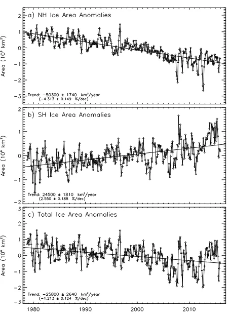
For completeness monthly sea ice area anomalies are presented in Figure 8 for the Arctic, the Antarctic and the combined regions. The distributions are very similar to those of the ice extents but not identical. The ice area monthly anomaly distribution shows a different record high anomaly occurring in 2007 in the Southern Hemisphere while the record high anomaly for ice extent in the same hemisphere occurred in 2014. This suggests that there was more divergence or large areas of low concentration ice in 2014 than in other years. The trends are also slightly different and shown to be -503,000 ± 17,400 km2 per decade (-4.31% per decade) for the Arctic, 245,000 ± 18, 100 km2 per decade (2.55% per decade) for the Antarctic and -258,000 ± 26,400 km2 per decade (-1.21% per
decade) for the global ice area.
Figure 8. Monthly anomaly of the sea ice area in (a) the Arctic; (b) the Antarctic; and (c) both hemispheres and linear regression
line that provides results of trend analysis.
The asymmetry in the trends for the two hemispheres has been considered counter intuitive because of direct observations of global warming (Hansen et al., 2010; Comiso and Hall, 2014). The difference in the geographical distribution of land and the ice cover in the two hemispheres likely contribute to the difference in the inter-annual variability in the sea ice distribution as well. It is however important to recognize that a trend in sea ice cover in the Arctic has implications that are different and likely more important than the observed trend in the Antarctic. In the Arctic, the sea ice cover is primarily in the Arctic Ocean basin where the surface temperature is extremely cold in winter and is surrounded by land that restricts expansion of the ice cover beyond the land boundary. In the summer the ice cover in the peripheral seas gets melted and the ones that survive are the thicker ice types that reside in the Arctic basin. The impact of ice-albedo feedback in the region is thus easier to evaluate since as the area of the ice that survives the summer gets smaller, there is more solar heat absorbed by larger areas of open water that in turn cause the mixed layer of water in the Arctic basin to warm up. Increases in the temperature of the mixed layer would cause less ice to survive the summer and the cycle is repeated. The net impact is a warmer Arctic that in turn makes the other components of the cryosphere in adjacent regions more vulnerable to change. This includes more reductions in the volume of the glaciers, less snow cover, thawing of the permafrost and the loss of mass in Greenland.
In the Antarctic the impact of ice albedo feedback is likely not as great because of large interannual variability in the location of summer ice and because of the more dynamic and larger
ocean environment that makes the change in mixed layer temperature associated with less (or more) summer ice very minimal.
The coldest region in the entire planet is located in the Eastern region of Antarctica where the temperature of the surface goes down to as low as about -80 ºC in the winter. The temperature of the sea ice cover that surrounds Antarctica is however considerably warmer because of lower latitude location and lower elevation. They are also considerably warmer than the sea ice cover in the Arctic region during the winter period. In addition to temperature, the extent of sea ice is also controlled by winds and ocean current that are also relatively strong in the region. The area of ice that survives the summer is relatively small as well and located unevenly on either sides of the Antarctic Peninsula. Since this ice gets advected out of the region during the winter period, the perennial ice cover in the Antarctic consists mainly of second year ice with normally unpredictable thickness.
3.2 Maximum and Minimum Extents
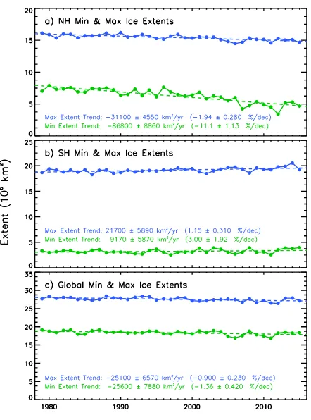
To gain insight into the state of the ice cover in the two hemispheres the yearly maximum and minimum ice extents are presented in Figure 9. The yearly maximum extents can provide the means to assess the influence of long-wave radiation, which is the dominant radiation during the winter period, on surface temperature. Ability to do this unambiguously, however, is not trivial because the changes in maximum extent are also influenced by other factors such as changes in atmospheric and ocean current circulation. In the Arctic, the maximimum extents were relatively uniform in the 1980s but started going down slowly during the subsequent years. The trend in maximum extent during the 37-year period is shown in Figure 5a to be about -1.94% per decade. In the 1980s, the Arctic basin region was almost all covered by ice at the end of the summer melt period because of the abundance of multiyear ice (or ice that survives at least two summers) which is the thick component and mainstay of the Arctic ice cover. In recent years, however, the perennial ice cover, represented by the ice cover during ice extent minimum in summer, has been reduced to less than half of what it was in the 1980s with a yearly trend of −11.1% per decade. The perennial ice includes multiyear ice which can be detected indirectly in winter by the sensor. The percentage decline in the multiyear ice extent is even larger which is about 13.5% per decade (Comiso 2012) and in addition, this ice type has been observed to be thinning (Kwok and Untersteiner 2011). The loss of this thick component of the sea ice cover would make the Arctic ice at the end of the summer vulnerable and the high rate of decline suggests that the Arctic basin might become totally ice free in a few decades unless a sustained cooling in the region occurs and the perennial sea ice cover recovers its previous thickness. The latter will not happen if the warming in the region as discussed in the next section continues. The occurrence of an ice free summer will be unprecedented and has been observed in the Arctic as recorded in human history for at least the last 1450 years (Kinnard et al., 2011). A disappearance would have profound effects on the climate, ecology, and environment not just of the region but also globally.
The trend of the sea ice cover in the Antarctic is in the opposite direction as indicated earlier but is relatively modest with the absolute value much less than that in the Arctic. The plots in Figure 9b indicate that yearly maximum extent in the region does not vary a lot with the trend estimated at only 1.15% per decade despite record high extents in winter in recent years.
The trend in minimum extent is a little higher at around 3.00% per decade suggesting the production of thicker ice during the growth period. Some studies indicate that the trend is related to more ice production owing to the decrease of ocean salinity in the region as a result of the melting of ice shelves (Jacobs et al. 2006). Others point out that a warming in the ocean would result in more evaporation that causes more solid precipitation over the region leading to colder surface temperature that enables higher rate in the growth of sea ice. A key observation is the increase in the dynamics of sea ice in the region and enhanced formation of coastal polynyas that serves as ice factories. Through modeling studies, it has been postulated that the increased dynamics might have been caused primarily by the occurrence of the ozone hole in recent years. The ozone hole apparently causes a deepening of the lows in the west Antarctic region which in turn leads to stronger southerly winds and higher ice production (Turner et al., 2009). Higher ice production in the more recent years has indeed been observed (Comiso et al., 2011; Martin et al., 2007).
The global maximum and minimum extents as presented in Figure 9c indicate overall decline with the trend in maximum extent being -0.90% per decade while that for the minimum extent being -1.36% per decade. Again, while the variability in the extent reflects that of the Antarctic data, the trends reflect the more dominant trends in the Arctic.
Figure 9. Yearly maximum and minimum extents of the sea ice cover in (a) the Arctic; (b) the Antarctic; and (c) the two hemispheres using a combined Arctic and Antarctic values.
4. CORRELATIONS WITH SURFACE TEMPERATURE AND ATMOSPHERIC CIRCULATION
4.1 Observed trends in surface temperature
Surface temperature is the primary parameter that determines the distribution of the sea ice cover. However, it is one of the most difficult to measure in situ consistently in the polar regions
because of extremely harsh and inhospitable conditions. Unattended sensors can also be buried by snow which is a good thermal insulator and cause large errors in the measurements. Reanalysis data (e.g., NCEP or ECMWF) have been used in modeling studies but such data have not been dependable in the polar regions because of the lack of adequate surface data as input. The data that have been most effective in characterizing the changes in surface temperature in the polar regions have been satellite data, especially thermal infrared data that provides coverage for both land and ocean regions. The time series that has been most frequently used has been those derived from Modeling studies has predicted amplification of global climate signals in the Arctic (Holland and Bitz, 2003). Observational studies using AVHRR data from August 1981 to July 2013 indeed indicates that the warming rate in the Arctic is more than three times the warming rate for the entire planet (Comiso and Hall, 2014). This phenomenon in part explains why the sea ice cover in the Arctic has been declining rapidly especially during the summer period. The asymmetry in the trend of sea ice cover the Arctic and the Antarctic has been the subject of many investigation. Modeling studies actually predicts a positive trend in the Antarctic which disagrees with the trends observed using satellite data.
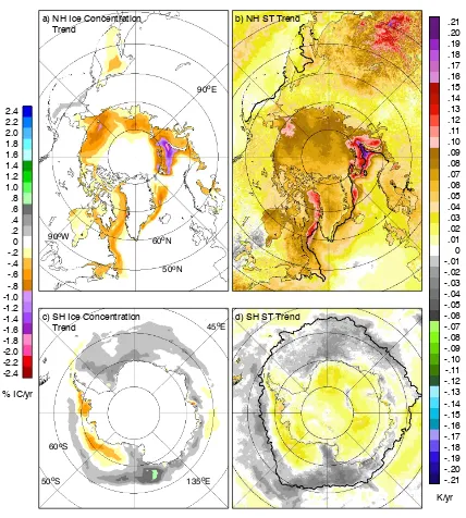
To gain insights into the sea ice asymmetry phenomenon trends in sea ice concentration and surface temperature in both Arctic and Antarctic regions are presented in Figure 10. Trends are estimated for each data element (pixel) using historical data for the period August 1981 to July 2015. The bold black line in the surface temperature maps represents the location of the 15% ice edge in 2014. The trend in ice concentration in the Arctic as positive in areas like Barents Sea, Beaufort Sea, Greenland Sea and Baffin Bay. The trend in ice concentration in the central Arctic where the perennial ice is usually located is minor and close to zero (white color) because the region is covered by ice most of the time even in summer while the trend in surface temperature over the same area is almost as high as in other areas of the Arctic. Such warming likely contributes to the thinning of the perennial ice cover.
The trends in ice concentration in the Antarctic are presented in Figure 10c. The trends in ice-covered regions are shown to be primarily positive except in some limited areas of the Bellingshausen Sea and Amundsen Sea. The latter seas have been the same regions where sea ice in the Antarctic has been declining (Comiso et al., 2011). The corresponding trend in surface temperature is shown in Figure 10d. Although the two images correspond to two independent measurements from two different sensors it is quite remarkable that the trends are consistently so similar but opposite in sign as expected. Areas where the sea ice concentration has been increasing as may be caused by longer ice growth season are also areas where the surface temperature have been declining. In the Bellingshausen
and Amundsen seas, the areas showing declines in sea ice are the same areas where surface temperature has been increasing.
It is apparent that the asymmetry in the trends of the sea ice cover in the two hemispheres is nicely reproduced in the surface temperature trends. The question is, how strong is the link between these two variables? The dramatic drop of sea ice cover in the Arctic in the summer of 2007 has been associated with a record high sea surface temperatures in the Beaufort Sea where the sea ice retreated the most during the year (Shibata et al., 2009). The result of correlation analysis of surface temperature and sea ice cover in the Arctic has yielded high correlation of the two variables (Comiso, 2003; Comiso, 2010). The correlation is not always strong because there are other environmental factors that could affect the distribution of the sea ice cover. For example, the record low extent of summer
Figure 10. Trends in surface temperature in the Arctic and the Antarctic
In the Southern Hemisphere, more quantitative analysis also yielded a strong connection of the two variables. Scatter plots of monthly averages of sea ice area versus surface temperature are presented in Figure 11 for the entire hemisphere and the various sectors. The plots all indicate high correlation values with the correlation coefficient for the entire Antarctic region estimated to be 0.94 while those for the various sectors are -0.90, -0.94, -0.92, -0.93 and -0.89 for the Weddell Sea, Indian Ocean, West Pacific Ocean, Ross Sea and Bellingshausen/ Amundsen Seas sectors, respectively.
Considering the spatial variability in the distribution of the trends of surface temperature worldwide it is thus not surprizing that the trends of the sea ice cover in the two hemispheres have opposite signs. While the observed trends of surface temperature in the Arctic indicate considerable warming warming rate that is more than 3 times that for global averages the observed trend of surface temperature in the Antarctic are
normally covered by sea ice. These results should suggest an asymmetry in the trends of sea ice cover in the two hemispheres considering the high correlation of the two variables.
Figure 11. Scatter plot of surface temperature versus sea ice area in the (a) Antarctic region and (b-f) the various Antarctic
sectors.
4.2 Correlations with Atmospheric Circulation
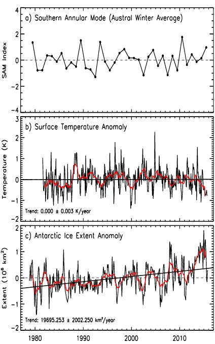
In addition to surface temperature the other factor that can cause significant changes in the trend of the sea ice cover is atmospheric circulation. In the Southern Hemisphere, the atmospheric circulation is governed mainly by the Southern Annular Mode (SAM) and is represented by SAM indices. The SAM index has been defined as the difference in the normalized monthly zonal-mean sea level pressure (SLP) between 40ºS and 65ºS (Thompson and Wallace, 2000). The SAM indices have been used to study the variability of and changes in the Antarctic sea ice cover (e.g., Kwok and Comiso, 2002; Gordon et al., 2010). To illustrate how the atmospheric pattern varied during the satellite era, austral winter SAM indices from November 1978 to 2015 are presented in Figure 12a. For comparative analysis, monthly anomalies of surface temperatures and sea ice extents are also shown in Figures 12b and 12c, respectively. Five month running averages are also provided (red line) in Figures 12b and 12c to improve ability to assess interannual patterns.
Periods of sustained negative values followed by sustained positive values (or vice-versa) are expected to cause significant changes in the atmospheric pattern that would cause sustained changes in the sea ice cover and surface temperature that in turn could cause the observed trends. The winter averages of SAM indices show large interannual variability but no sustained patterns nor a significant trend. It is also apparent that the location of the dips and peaks in the three plots do not normally match with a few exceptions. For example, a dip in the SAM index in 2002 correspond to a dip in surface temperature anomaly and a peak in ice extent anomaly. In a few cases two parameters would match but the third one would not. However, generally the correlation is not good with the correlation coefficient close to zero.
Figure 12. (a) Yearly averages of the Southern Hemisphere Annular Mode indices during the winter period and monthly (b) surface temperature and (c) sea ice extent anomalies from 1978
to 2015.
In the Arctic, the atmospheric circulation is dominated by the Arctic Oscillation which is more formally referred to as Northern Hemisphere Annular Mode (NAM). To get an idea about longer term behaviour, winter and annual AO indices data for 65 years from 1950 to 2015 are plotted in Figure 13. In this case a discernable pattern is revealed with the indices generally negative up to around 1986 and mostly positive after that. In the 1990s the negative indices were associated with high extents in the sea ice cover while the positive indices were associated with low extents. It appears the the indices went almost neutral in the late 1990s, as noted by Overland and Wang (2005), and there were examples of very negative episodes as in 2010 that were not coherent with the pattern of the sea ice cover. Also, the high values in early 1990s and the low values in 1979 and 1986 do not correspond to abnormal changes in the sea ice cover. There were also postulates that a reversal of the sign of the AO index means a reversal in the atmospheric circulation pattern (e.g., from cyclonic to anti-cyclonic circulation). This postulate was not consistent with observations as well.
For comparison, the SST measurements during the same period are presented in Figure 13b. Because of the lack of satellite data in the early periods the SST data used for this comparison is the historical in situ measurements as described by Reynolds et al. (2002). No comparable data about ice extent during the period exist. The plot looks interesting in that from the late 1980s when the perennial sea ice cover started to go down, the SST was going up. This again is a strong manifestation of the strong link of SST with the sea ice cover.
Figure 13. (a) winter and annual indices of the Arctic Oscillation from a950 to 2015 and (b) SST anomalies in the
Arctic region for the same period.
5. Research Initiatives to Address the Future State of the Sea Ice Cover
The observed declines in the perennial ice cover in the late 1990s have led to several initiatives to address the future of the sea ice cover. One of them is an international project called SHEBA in 1997-1998 in which a research ship was kept in the Arctic over a whole year to enable scientists to directly observe the current state of the Arctic sea ice cover. Similar projects are planed for the future. There has also been a lot of field work to look at not just the physical changes but also the biological changes in both marine (e.g., Distributed Biological Observatory, DBO) and land (Yamal Project) to better understand the impact of the receding ice to the ecology and productivity of the region. During the International Polar Year from 2007 to 2008 many countries did collaborative work and collected a lot of data about the Arctic Climate System. The awareness of the seriousness of the problems associated with the changing Arctic has increase tremendously in the recent decade and this led to the formation of many international and national committees and panels to address some of the issues.
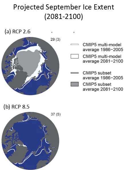
IPCC 2014 has reported through the use of CMIPS 5 (Coupled Model Intercomparison Project, version 5) the difference in the projections of the sea ice cover for the year 2081 to 2100 for two different Representative Concentration Pathways (RCP). Two scenarios, namely: RCP 2.6 and RCP 8.5, are presented in Figure 14. In RCP 2.6, the anthropogenic contribution to greenhouse gases is maintained constant at near current conditions and the sea ice cover would not change much from the present. On the other hand, in RCP 8.5, which allows the anthropogenic contribution to continue to rise at the current rate, the perennial ice cover would completely disappear. The possibility of preventing further decline in the perennial ice
under RSP 2.6 is encouraging but more research is needed to improve the accuracy in the projections.
Figure 14. Modeling results of the future of the sea ice cover in the Arctic with (a) continued increase in greenhouse gases and
(b) keeping the greenhouse gases at the same level as it is at present. (Courtesy of IPCC 2014)
6. Discussion and Conclusions
The ability to monitor and quantify changes in the Arctic and Antarctic sea ice cover has been considerably enhanced through the use of data from high performance satellite systems. We now know for sure that there is an asymmetry in the trends of sea ice in the two hemispheres. In this study we show that there is a similar asymmetry in the trends of surface temperature and there is a strong correlation of changes in sea ice cover with changes in surface temperature. The observed asymmetry is thus not too unusual and should even be expected. Overall, the global warming rate is relatively small compared to that of the Arctic. But when ice cover data from both hemispheres are combined the net trend in the ice cover is also relatively small and consistent with the warming rate for the entire globe.
The observed amplification of surface temperature in the Arctic is consistent with the rapid decline in the sea ice cover in the summer. It is also consistent with modeling studies that includes the effect of ice-albedo feedbacks. The retreat of sea ice and 2011, it started to decline again and a record low was observed in 2012. The drastic decline in 2007 was accompanied by unusually warm sea surface temperature in the Beaufort Sea region (Shibata et al., 2010). The record low ice cover in 2012 was not accompanied by anomalously high sea surface
temperature but was in part caused by an unusually strong storm during the middle of summer (Parkinson and Comiso, 2013). There was again a recovery of summer ice in 2013, 2014 and 2015. The question is what causes the recovery? If ice albedo feedback causes a conditioning and a general warming of the region, what is the general mechanism that enables the sea ice cover in the Arctic region to recover? Similarly, in the Antarctic, the ice extent was a record high in 2014 but was not sustained in 2015 despite good monthly agreement of the ice cover for the two years up to June. What is unusual in the environmental conditions that led to high extents in 2014 but relatively low extent in 2015? Changes in the atmospheric circulation system could help resolve the issues but a comparative study with the Arctic Oscillation indices in the Arctic and SAM indices in the Antarctic do not yield any strong correlation with the changes in the sea ice cover. These are questions that requires more research and should be well understood to enable accurate projections on the future of the sea ice cover.
ACKNOWLEDGEMENTS
The author is grateful to Robert Gersten of ADNET and Larry Stock of SGT both working at NASA/Goddard Space Flight Center for programming and analysis support. Funds for the project was provided by the Cryopheric Sciences Program at NASA Headquarters.
REFERENCES
Bhatt, U. S., D. A. Walker, M. K. Raynolds, P. A. Bienick, H. E. Epstein, J. C. Comiso, J. E. Pinzon, C. J. Tucker, and I. V. Polyakov, 2013. Recent declines in warming and vegetation greening trends over Pan-Arctic Tundra, Remote Sensing, 5, pp 4229-4254, doi: 10.3390/rs5094229.
Cavalieri DJ, Gloersen P, Campbell WJ (1984) Determination of sea ice parameters with the Nimbus 7 SMMR. J. Geophys Res 89, pp. 5355-5369.
Cavalieri, D.J., P. Gloersen, C. Parkinson, J. Comiso, and H.J. Zwally, 1997. Observed hemispheric asymmetry in global sea ice changes, Science,278(7), pp. 1104-1106.
Cavaliers, D. J., and C. L. Parkinson, 2012. Arctic sea ice variability and trends, 1979-2010. The Cryosphere, 6, pp. 881-889, doi:10.5194/tc-6881-2012.
Comiso, J. C., 1986. Characteristics of winter sea ice from satellite multispectral Microwave observations. J. Geophys.
Rev., 91(C1), pp. 975-994.
Comiso, J. C., 2003. Warming Trends in the Arctic, J. Climate, 16(21), pp. 3498-3510.
Comiso, J.C., 2010. Polar Oceans from Space. Springer Publishing, New York, 495pp.,doi10.1007/978-0-387- 68300-3.
Comiso, J. C. and D. K. Hall, 2014. Climate Trends in the Arctic, WIREs (Wiley Interdisciplinary Reviews) Climate
Change, Advanced Review: doi:10.1002/wcc.277.
Comiso, J. C., 2002. A rapidly declining Arctic perennial ice cover, Geophys Res. Letts., 29(20), 1956, doi:10.1029/
2002GL015650.
Comiso, J. C. and F. Nishio, 2008. Trends in the sea ice cover using enhanced and compatible AMSR-E, SSM/I and SMMR data. J. Geophys. Res. 113, C02S07, doi:10.1029/ 2007JC004257.
Comiso, J. C., C. L. Parkinson, R. Gersten, and L. Stock, 2008. Accelerated decline in the Arctic sea ice cover, Geophys. Res.
Lett., 35, L01703,doi:10.1029/2007GL031972.
Comiso, J. C., R. Kwok, S. Martin and A. Gordon, 2011. Variability and trends in sea ice and ice production in the Ross Sea. J. Geophys. Res., 116, C04021, doi:1029/2010JC006391. Fletcher, J.O., and J.J. Kelley. 1978. “The Role of the Polar Regions in Global Climate Change.” In Polar Research: To the
Present, and the Future, edited by M.A. McWhinnie. Boulder,
CO: Westview Press.
Gordon, A. L., and J. C. Comiso, 1988. Polynyas in the Southern Ocean, Scientific American, 256, pp. 90-97.
Gordon, A.L., M. Visbeck, and J.C. Comiso, 2007. A link between the Great Weddell Polynya and the Southern Annular Mode, J. Climate, 20(11), pp. 2558-2571.
Hansen, J., R. Ruedy, M. Sato, and K. Lo, 2010. Global surface temperature change, Rev. Geophys., 48, RG4004, doi:10.1029/2010RG000345.
Holland, M. M., and C. M. Bitz, 2003. Polar amplification of climate change in courpled models, Clim. Dyn., 23, pp. 221-232.
Holland, P. R., and R. Kwok, 2012. Wind-driven trends in Antarctic sea-ice drift, Nature Geoscience, 5, pp. 872-875.
IPCC. 2014. “Summary for Policymakers.” In Climate Change
2013: The Physical Basis. Contribution of Working Group I to
the Fifth Assessment Report of the Intergovernmental Panel on Climate Change, edited by T.F. Stocker, D. Qin, G.K. Plattner,
et al. Cambridge: Cambridge University Press.
Jacobs, S. S., 2006. Observations of change in the Southern Ocean, Phil. Trans. Royal Soc., 364, pp. 1657-1681, doi:10.1098/rsta.2006.1794.
Jacobs, S.S., and J.C. Comiso, 1997. Climate variability in the Amundsen and Bellingshausen Seas, J. Climate, 10(4), pp. 697-709.
Kwok, R., and J. C. Comiso, 2002. Spatial patterns of variability in Antarctic surface temperature: Connections to the Southern Hemisphere Annular Mode and the Southern Oscillation, Geophys. Res. Lett., 29(14), doi:10.1029/ 2002GL015415.
Kwok, R., and N. Untersteiner. 2011. “The Thinning of Arctic Sea Ice.” Physics Today, 64, pp. 36–41.
Luthcke, S. B., and Coauthors, 2006. Recent Greenland ice mass loss by drainage system from satellite gravity observations, Science, 314, pp.1286–1289.
Markus, T. and D.J. Cavalieri, 2009. The AMSR-E NT2 Sea ice concentration algorithm: its basis and implementation. Remote
Sensing Soc. of Japan, 29(1), pp.216-223.
Martin, S., R.S. Drucker and R. Kwok, 2007. The areas and ice production of the western and central Ross Sea polynyas, 1992-2002, and their relation to the B-15 and C-19 iceberg events of 2000 and 2002. J. Marine Systems, 68, pp. 201-214.
Overland, J.E., and M. Wang. 2005. “The Arctic Climate Paradox: The Recent Decrease of the Arctic Oscillation.”
Geophysical Research Letters, 32(6). DOI:10.1029/
2004GL021752.
Reynolds, R.W., N.A. Rayner, T.M. Smith, et al. 2002. “An Improved in Situ and Satellite SST Analysis of Climate.”
Journal of Climate, 15, pp. 1609–1625.
Shibata, A., H. Murakami, and J. Comiso, 2010. Anomalous Warming in the Arctic Ocean in the Summer of 2007, J. Remote
Sensing Society of Japan, 30(2), pp. 105-113.
Smith, Jr. W., and J. C. Comiso, 2008. The influence of sea ice primary production in the Southern Ocean: A satellite perspective, J. Geophys. Res.,113, C05S93, doi:10.1029/ 2007JC004251.
Steffen, K., D. J. Cavalieri, J. C. Comiso, K. St. Germain, P. Gloersen, J. Key, and I. Rubinstein, 1992. "The estimation of geophysical parameters using Passive Microwave Algorithms," Chapter 10, Microwave Remote Sensing of Sea Ice, (ed. by Frank Carsey), American Geophysical Union, Washington, D.C., pp. 201-231.
Swift, C.T., L.S. Fedor, and R.O. Ramseier, 1985. An algorithm to measure sea ice concentration with microwave radiometers, J. Geophys. Res., 90(C1), pp.1087-1099.
Thompson, D. W. J., and J. M. Wallace, 2000. Annular modes in the extratropical circulation. Part I: Month-to-month variability. J. Climate, 13, pp. 1000-1016.
Turner, J., J.C. Comiso, G. J. Marshall, T.A. Lachlan-Cope, T. Bracegirdle, T. Maksym, M. Meredith and Z. Wang, 2009. Non-annular atmospheric circulation change induced by stratospheric ozone depletion and its role in the recent increase of Antarctic sea ice extent, Geophy. Res. Lett. 36, L08502, doi:10.1029/ 2009GL037524.
Vant MR, Gray RB, Ramseier RO, Makios V., 1974. Dielectric properties of fresh and sea ice at 10 and 35 GHz, J. Applied Physics, 45(11), pp. 4712-4717
Wang, X., and J. Key, 2003. Recent trends in Arctic surface, cloud, and radiation properties from space, Science, 299, pp. 1725–1728.
Zwally, H. J., W. Abdalati, T. Herring, K. Larson, J. Saba, K. Steffen, 2002. Surface melt-induced acceleration of Greenland Ice-Sheet Flow, Science, 297, pp. 218-222.