SNOW DEPTH ESTIMATION USING TIME SERIES PASSIVE MICROWAVE
IMAGERY VIA GENETICALLY SUPPORT VECTOR REGRESSION
(CASE STUDY URMIA LAKE BASIN)
Zahir Nikraftar ª, and Mahdi Hasanlou ª
ª University of Tehran, College of Engineering, School of Surveying and Geospatial Engineering., Tehran,
Iran;[email protected] , [email protected]
KEY WORDS: Urmia Basin, Snow Depth, Support Vector Regression, Wavelet Denoising, Genetic Algorithm, band reduction
ABSTRACT:
Lake Urmia is one of the most important ecosystems of the country which is on the verge of elimination. Many factors contribute to this crisis among them is the precipitation, paly important roll. Precipitation has many forms one of them is in the form of snow. The snow on Sahand Mountain is one of the main and important sources of the Lake Urmia’s water. Snow Depth (SD) is vital parameters for estimating water balance for future year. In this regards, this study is focused on SD parameter using Special Sensor Microwave/Imager (SSM/I) instruments on board the Defence Meteorological Satellite Program (DMSP) F16. The usual statistical methods for retrieving SD include linear and non-linear ones. These methods used least square procedure to estimate SD model. Recently, kernel base methods widely used for modelling statistical problem. From these methods, the support vector regression (SVR) is achieved the high performance for modelling the statistical problem. Examination of the obtained data shows the existence of outlier in them. For omitting these outliers, wavelet denoising method is applied. After the omission of the outliers it is needed to select the optimum bands and parameters for SVR. To overcome these issues, feature selection methods have shown a direct effect on improving the regression performance. We used genetic algorithm (GA) for selecting suitable features of the SSMI bands in order to estimate SD model. The results for the training and testing data in Sahand mountain is [R²_TEST=0.9049 and RMSE= 6.9654] that show the high SVR performance.
INTERODUCTION
Sahand mountain that is located in the vicinity of lake Urmia it is geographical coordinates are in eastern direction from 45°57'31.44"E to 46°44'29.70"E and in northern direction from 37°22'41.90"N to 38°2'15.49"N. The snow on this mountain is one of the main and important sources of the Urmia Lake water. Therefore monitoring and studying of this parameter is crucial. For studying the snow, we must investigate the main factors of the snow including, the snow depth (SD), density of the snow, the snow water equivalent (SWE) and etc. The common methods of calculating the SD are include incorporating in situ observations and using satellite remote sensing observations. The in situ observation method is an accurate method but it is hazardous in mountain region. Another’s short coming of this method is that it cannot cover the whole area and also the low density coverage of the area. The usual procedure for incorporating remote sensing imageries to estimate SD is utilizing passive microwave domain in electromagnetic spectrum. The most suitable bands for this domain located in 19 to 81GHz. One of the newest sensor which takes images in this range is DMSP F16-SSM/IS. This sensor takes images in two modes – IMAGER (SSMI) and SOUNDER (SSMS) (“National Climatic Data Center (ncdc) | Climate Data Records (cdr) Program,” n.d.). In his paper, datasets from SSMI mode are used. The IMAGER datasets of this sensor has seven bands in four wavelengths and respectively they are inter calibrated. Nowadays, passive microwave remote sensing is the most efficient way to derive snow depth at global and regional scales(Sturm et al., 2010; Tedesco and Narvekar, 2010). Snow-depth algorithms were
developed using a brightness temperature difference of 18–37 GHz (Foster et al., 1997) and single band temperature (Matkan, 2003). Tao CHE adopt Grody’s decision-tree method to obtain snow cover from SMMR (1978–87) and SSM/I and then they modified change algorithm before regression, the adverse factors, such as liquid-water content within the snowpack, forest, lakes, was taken into account. To assess the accuracy of snow depth retrieved from the modified algorithm, they used measured SD data at the meteorological stations in 1983 and 1984 to compare with the SMMR results, and those in 1993 for the SSM/I results. The two absolute errors less than 5cm hold about 65% of all the data. The standard deviations are 6.03cm and 5.61cm for SMMR and SSM/I, respectively (Che et al., 2008). Using the Chang algorithm in the global scale, it was shown that a single algorithm cannot describe all the different kinds of snow conditions (Foster et al., 1997). The SD that is retrieved by a nonlinear data mining technique, the modified sequential minimal optimization (SMO) algorithm for support vector machine (SVM) regression using SSM/I and SSM/R andvisible/infrared surface reflectance from Moderate Resolution Imaging Spectroadiometer (MODIS) products. The proposed method is tested by using 16,329 records of dry snow measured at 54 meteorological stations in Xinjiang, China over an area of 1.6 million km2 from 2000 to 2009. The root mean square error (RMSE), relative RMSE and the correlation coefficient of this method are 6.21 cm, 0.64 and 0.87, respectively. These results was better than those obtained using only brightness temperature data (8.80 cm, 0.90 and 0.73), the traditional spectral polarization difference (SPD) The International Archives of the Photogrammetry, Remote Sensing and Spatial Information Sciences, Volume XL-1/W5, 2015
International Conference on Sensors & Models in Remote Sensing & Photogrammetry, 23–25 Nov 2015, Kish Island, Iran
This contribution has been peer-reviewed.
algorithm (15.07 cm, 1.54 and 0.58), a modified Chang algorithm in WESTDC (9.80 cm, 1.00 and 0.62), or the multilayer perceptron classifier of artificial neural networks (ANN) (9.23 cm, 0.94 and 0.72). The daily snow water equivalent (SWE) retrieved by this method has an RMSE of 8.05 mm and a correlation of 0.84, which are better than those of NASA NSIDC (32.87 mm and 0.47) or Glob snow (19.07mmand 0.59) (Liang et al., 2015). In the other algorithms single band or double bond have been used for snow depth retrieval from SSM/I data. In this study we implement SVR using RBF kernel and try to tuning RBF parameter’s and then using these parameters Genetically-SVR was implement on datasets. With this method not only parameters has been tuned also the band/feature selection with this method is tuned too. The datasets used in this paper is provided from ground station and SSM/I passive microwave data from 2007 to 2013. In situ data achieved from Iranian Water Resource Management Company for these dates.
1-METHODOLOGY
By examining the obtained data from SSM/I TB band and in situ snow depth show, it is revealed that our datasets suffering from noise. For this reason we used wavelet denoising method for eliminating these noises. The most of previous mentioned methods used one band or dual-band microwave passive combinations. These methods are used simple linear relations between bands. The proposed method in this paper is distinguish from the other method because its ability for selecting the bests and appropriate bands from the seven input bands while it’s may be more than one or two.
1.1 Support Vector Regression
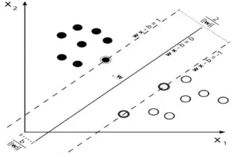
The original SVM algorithm was invented by Vladimir N. Vapnik and Alexey Ya. Chervonenkis in 1963. Vapnik suggested a way to create nonlinear classifiers by applying the kernel trick to maximum-margin hyper planes (Boser et al., 1992). The current standard incarnation (soft margin) was proposed by Corinna Cortes and Vapnik in 1993 and published in 1995 (Cortes and Vapnik, 1995). More formally, a support vector machine constructs a hyper plane or set of hyper planes in a high or infinite dimensional space, which can be used for classification, regression, or other tasks. Intuitively, a good separation is achieved by the hyper plane that has the largest distance to the nearest training-data point of any class (so-called functional margin), since in general the larger the margin the lower the generalization error of the classifier. SVR method in the past decade known as one of the reliable and efficient methods. In machine learning, SVMs are supervised learning models which associate with learning algorithm used for classification and regression analysis. The original SVM algorithm was introduced by Vapnik. Scholkopf and Smola proposed a more in-depth overview of SVM regression (Scholkopf and Smola, 2001). SVR for classifying or regression of the multidimensional features takes the data in to higher dimension and using quadratic programing to solve the equation and reduce maximum margin in results (Fige.1). The results of this method in addition to high accuracy has a stability too.
Figure 1. Maximum-margin hyper plane and margins for an SVM trained with samples from two classes (Samples on the
margin are called the support vectors).
1.2 Feature Selection Based ON Genetic Algorithm
1.2.1 Feature Selection
Feature selection is the process of identifying and removing from a training data set as much irrelevant and redundant features as possible. This, reduces the dimensionality of the data and may enable regression algorithms to operate faster and more effectively. In some cases, correlation coefficient can be improved; in others, the result is a more compact, easily interpreted representation of the target concept.
1.2.2 Genetic Algorithm
Genetic Algorithms (GA) are search algorithms inspired by evolution and natural selection, and they can be used to solve different and diverse types of problems. The algorithm starts with a group of individuals (chromosomes) called a population. Each chromosome is composed of a sequence of genes that would be bits, characters, or numbers. Reproduction is achieved using crossover (2 parents are used to produce 1 or children) and mutation (alteration of a gene or more). Each chromosome is evaluated using a fitness function, which defines which chromosomes are highly-fitted in the environment. The process is iterated for multiple times for a number of generations until optimal solution or maximum iteration is reached. (Figure 2) The reached solution could be a single individual or a group of individuals obtained by repeating the GA process for many runs.
Figure 2. GA steps
The International Archives of the Photogrammetry, Remote Sensing and Spatial Information Sciences, Volume XL-1/W5, 2015 International Conference on Sensors & Models in Remote Sensing & Photogrammetry, 23–25 Nov 2015, Kish Island, Iran
This contribution has been peer-reviewed.
DATA SETS
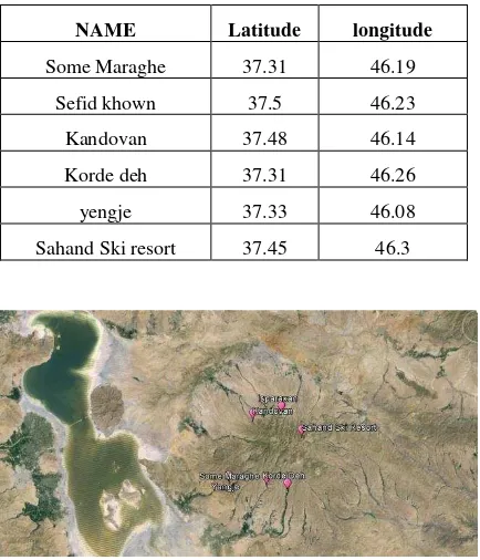
In situ measurement is obtained in the period of years 2007 to 2013 at five station in Sahand Mountain that in this region does not exist any forest, lake or other adverse factors. The SSM/I data was provided from NOAA national climate data center (NCDC, 1963). Geographic coordinate and visually display of these stations is respectively shown in Table (1) and Figure (4).
TABLE (1) Ground station name and coordinates
Figure (4). Visually display of stations in the vicinity of Urmia Lake
As mentioned later, we applied wavelet denoising using daubechies wavelet for noise removal from datasets. Figure (5) show the standard deviation from mean for each band before and after denoising procedure.
Figure (5). STD for incorporated bands before and after wavelet denoising method
Then denoised datasets has been take to multidimensional space using SVR by RBF kernel. There are two parameters for an RBF kernel C and γ that should be determined. On the other hands, There are two kind of model selection (parameter search) exist for determining C and γ. Cross -validation (CV) and search (GS) that we use Grid-search method in this paper. Now we should remove redundant bands that reduce accuracy of the model. It should be note in the previous stage 40 percent of the data’s considered to training data and the left 60 percent as a test data’s. The determined parameters remind fix for next phases. Then we used Genetic Algorithm (GA) combined with SVR for determining the best bands/features for retrieving SD. In the each iteration a new selection of band that chosen by GA from denoised data and fixed parameters get into the SVR then MSE and R square has been determined. Figure (6) show the genetically _ SVR that was converged.
Figure (6). GA_SVR converged
In the previous phase, band 19H and band 81H has been considered as a best bands for SD retrieving (Eq 1).
�� = � ����1 �, ���� 1� 1
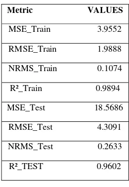
Figure (5) show the convergence of the model. Table (2) show the MSE, RMSE, Normalized RMSE and R-square for train and test data set at the end the model that Obtained from previous phases has been apply on the mentioned region and SD model was obtained Figure (7).
0
5 10 15 20 25
STD B19V
STD B19H
STD B22V
STD B37V
STD B37H
STD B81V
STD B81H
Before denoising after denoising
NAME Latitude longitude
Some Maraghe 37.31 46.19
Sefid khown 37.5 46.23
Kandovan 37.48 46.14
Korde deh 37.31 46.26
yengje 37.33 46.08
Sahand Ski resort 37.45 46.3
The International Archives of the Photogrammetry, Remote Sensing and Spatial Information Sciences, Volume XL-1/W5, 2015 International Conference on Sensors & Models in Remote Sensing & Photogrammetry, 23–25 Nov 2015, Kish Island, Iran
This contribution has been peer-reviewed.
Table (2). Resulted of the model
Figure (7). Snow Depth model derived
DISCUSSION
Based on the results and unlike other method that just used lower band, it has been shown, by combining of GA algorithm and kernel based method (SVR) it is possible to used new band combination and reach to a most efficient results. These results is yield from 40 time iteration of the algorithm and it is robust. It should be considered that our datasets is in regional scale and maybe if we use dataset in global scale than better will be achieved.
CONCLUSION
This study proposed a method to snow depth retrieval algorithm from SSM/I passive microwave data. The results show that this algorithm is reliable to obtain desired information with high accuracy and high performance with R²=0.96. This method is able to use different band combination using genetic algorithm and get this band in to SVR algorithm and then solve the problem in space with higher dimension. Then by combination of the genetic algorithm and support vector regression and tuning of these parameters, reached to a new band combination with high
performance in SD retrieval. The results is from 40 time iteration of the algorithm and is robust. These datasets is in the regional scale and we suggest for the future work to implement this method on the global scale to achieve global model with high performance.
REFRENCES
Boser, B.E., Guyon, I.M., Vapnik, V.N., 1992. A training algorithm for optimal margin classifiers, in: Proceedings of the Fifth Annual Workshop on Computational
Learning Theory. ACM, pp. 144–152.
Che, T., Xin, L., Jin, R., Armstrong, R., Zhang, T., 2008. Snow depth derived from passive microwave remote-sensing data
in China. Ann. Glaciol. 49, 145–154.
Cortes, C., Vapnik, V., 1995. Support-vector
networks. Mach. Learn. 20, 273–297.
Foster, J.L., Chang, A.T.C., Hall, D.K., 1997. Comparison of snow mass estimates from a prototype passive microwave snow algorithm, a revised algorithm and a snow depth climatology. Remote
Sens. Environ. 62, 132–142.
Liang, J., Liu, X., Huang, K., Li, X., Shi, X., Chen, Y., Li, J., 2015. Improved snow depth retrieval by integrating microwave brightness temperature and
visible/infrared reflectance. Remote
Sens. Environ. 156, 500–509.
Matkan, A.A., 2003. Snow Depth Estimation in Iran, Using: DMSP F11-SSM/I Satellite
Data. Geogr.-Sientific J. IGA 8–27.
National Climatic Data Center (ncdc) | Climate Data Records (cdr) Program [WWW Document], n.d. URL
http://www.ncdc.noaa.gov/cdr/operation alcdrs.html#4 (accessed 9.3.15). Scholkopf, B., Smola, A.J., 2001. Learning with
kernels: support vector machines, regularization, optimization, and beyond. MIT press.
Sturm, M., Taras, B., Liston, G.E., Derksen, C., Jonas, T., Lea, J., 2010. Estimating snow water equivalent using snow depth data and climate classes. J.
Hydrometeorol. 11, 1380–1394.
Tedesco, M., Narvekar, P.S., 2010. Assessment of the NASA AMSR-E SWE Product. Sel. Top. Appl. Earth Obs. Remote
Sens. IEEE J. Of 3, 141–159.
Metric VALUES
MSE_Train 3.9552
RMSE_Train 1.9888
NRMS_Train 0.1074
R²_Train 0.9894
MSE_Test 18.5686
RMSE_Test 4.3091
NRMS_Test 0.2633
R²_TEST 0.9602
The International Archives of the Photogrammetry, Remote Sensing and Spatial Information Sciences, Volume XL-1/W5, 2015 International Conference on Sensors & Models in Remote Sensing & Photogrammetry, 23–25 Nov 2015, Kish Island, Iran
This contribution has been peer-reviewed.