Chicago, IL 60606-6412 Tel: (312) 651-3000 Fax: (312) 651-3668
SPSS is a registered trademark and the other product names are the trademarks of SPSS Inc. for its proprietary computer software. No material describing such software may be produced or distributed without the written permission of the owners of the trademark and license rights in the software and the copyrights in the published materials.
The SOFTWARE and documentation are provided with RESTRICTED RIGHTS. Use, duplication, or disclosure by the Government is subject to restrictions as set forth in subdivision (c) (1) (ii) of The Rights in Technical Data and Computer Software clause at 52.227-7013. Contractor/manufacturer is SPSS Inc., 233 South Wacker Drive, 11th Floor, Chicago, IL 60606-6412.
Patent No. 7,023,453
General notice: Other product names mentioned herein are used for identification purposes only and may be trademarks of their respective companies.
Windows is a registered trademark of Microsoft Corporation.
Apple, Mac, and the Mac logo are trademarks of Apple Computer, Inc., registered in the U.S. and other countries.
This product uses WinWrap Basic, Copyright 1993-2007, Polar Engineering and Consulting,http://www.winwrap.com.
Printed in the United States of America.
No part of this publication may be reproduced, stored in a retrieval system, or transmitted, in any form or by any means, electronic, mechanical, photocopying, recording, or otherwise, without the prior written permission of the publisher.
ISBN-13: 978-1-56827-401-0 ISBN-10: 1-56827-401-7
TheSPSS Statistics 17.0 Brief Guideprovides a set of tutorials designed to acquaint you with the various components of SPSS Statistics. This guide is intended for use with all operating system versions of the software, including: Windows, Macintosh, and Linux. You can work through the tutorials in sequence or turn to the topics for which you need additional information. You can use this guide as a supplement to the online tutorial that is included with the SPSS Statistics Base 17.0 system or ignore the online tutorial and start with the tutorials found here.
SPSS Statistics 17.0
SPSS Statistics 17.0 is a comprehensive system for analyzing data. SPSS Statistics can take data from almost any type offile and use them to generate tabulated reports, charts, and plots of distributions and trends, descriptive statistics, and complex statistical analyses.
SPSS Statistics makes statistical analysis more accessible for the beginner and more convenient for the experienced user. Simple menus and dialog box selections make it possible to perform complex analyses without typing a single line of command syntax. The Data Editor offers a simple and efficient spreadsheet-like facility for entering data and browsing the working datafile.
Internet Resources
The SPSS Inc. Web site (http://www.spss.com) offers answers to frequently asked questions and provides access to datafiles and other useful information.
In addition, the SPSS USENET discussion group (not sponsored by SPSS Inc.) is open to anyone interested . The USENET address iscomp.soft-sys.stat.spss.
You can also subscribe to an e-mail message list that is gatewayed to the USENET group. To subscribe, send an e-mail message to[email protected]. The text of the e-mail message should be:subscribe SPSSX-L firstname lastname. You can then post messages to the list by sending an e-mail message to[email protected].
Logistic Regression and General Linear Models. TheAdvanced Statistical Procedures Companionhas also been published by Prentice Hall. It includes overviews of the procedures in the Advanced and Regression modules.
SPSS Statistics Options
The following options are available as add-on enhancements to the full (not Student Version) SPSS Statistics Base system:
Regressionprovides techniques for analyzing data that do notfit traditional linear statistical models. It includes procedures for probit analysis, logistic regression, weight estimation, two-stage least-squares regression, and general nonlinear regression.
Advanced Statisticsfocuses on techniques often used in sophisticated experimental and biomedical research. It includes procedures for general linear models (GLM), linear mixed models, variance components analysis, loglinear analysis, ordinal regression, actuarial life tables, Kaplan-Meier survival analysis, and basic and extended Cox regression.
Custom Tablescreates a variety of presentation-quality tabular reports, including complex stub-and-banner tables and displays of multiple response data.
Forecastingperforms comprehensive forecasting and time series analyses with multiple curve-fitting models, smoothing models, and methods for estimating autoregressive functions.
Categoriesperforms optimal scaling procedures, including correspondence analysis.
Conjointprovides a realistic way to measure how individual product attributes affect consumer and citizen preferences. With Conjoint, you can easily measure the trade-off effect of each product attribute in the context of a set of product attributes—as consumers do when making purchasing decisions.
Exact Testscalculates exactpvalues for statistical tests when small or very unevenly distributed samples could make the usual tests inaccurate. This option is available only on Windows operating systems.
Missing Valuesdescribes patterns of missing data, estimates means and other statistics, and imputes values for missing observations.
Decision Treescreates a tree-based classification model. It classifies cases into groups or predicts values of a dependent (target) variable based on values of independent (predictor) variables. The procedure provides validation tools for exploratory and confirmatory classification analysis.
Data Preparationprovides a quick visual snapshot of your data. It provides the ability to apply validation rules that identify invalid data values. You can create rules thatflag out-of-range values, missing values, or blank values. You can also save variables that record individual rule violations and the total number of rule violations per case. A limited set of predefined rules that you can copy or modify is provided.
Neural Networkscan be used to make business decisions by forecasting demand for a product as a function of price and other variables, or by categorizing customers based on buying habits and demographic characteristics. Neural networks are non-linear data modeling tools. They can be used to model complex relationships between inputs and outputs or tofind patterns in data.
EZ RFMperforms RFM (receny, frequency, monetary) analysis on transaction datafiles and customer datafiles.
Amos™(analysis ofmomentstructures) uses structural equation modeling to confirm and explain conceptual models that involve attitudes, perceptions, and other factors that drive behavior.
Training Seminars
SPSS Inc. provides both public and onsite training seminars for SPSS Statistics. All seminars feature hands-on workshops. seminars will be offered in major U.S. and European cities on a regular basis. For more information on these seminars, contact your local office, listed on the SPSS Inc. Web site athttp://www.spss.com/worldwide.
Technical Support
Technical Support services are available to maintenance customers of SPSS Statistics. (Student Version customers should read the special section on technical support for the Student Version. For more information, seeTechnical Support for Studentson p. vii.) Customers may contact Technical Support for assistance in using products or for
yourself, your organization, and the serial number of your system.
SPSS Statistics 17.0 for Windows Student Version
The SPSS Statistics 17.0 for Windows Student Version is a limited but still powerful version of the SPSS Statistics Base 17.0 system.
Capability
The Student Version contains all of the important data analysis tools contained in the full SPSS Statistics Base system, including:
Spreadsheet-like Data Editor for entering, modifying, and viewing datafiles.
Statistical procedures, includingttests, analysis of variance, and crosstabulations.
Interactive graphics that allow you to change or add chart elements and variables dynamically; the changes appear as soon as they are specified.
Standard high-resolution graphics for an extensive array of analytical and presentation charts and tables.
Limitations
Created for classroom instruction, the Student Version is limited to use by students and instructors for educational purposes only. The Student Version does not contain all of the functions of the SPSS Statistics Base 17.0 system. The following limitations apply to the SPSS Statistics 17.0 for Windows Student Version:
Datafiles cannot contain more than 50 variables.
Datafiles cannot contain more than 1,500 cases. SPSS Statistics add-on modules (such as Regression or Advanced Statistics) cannot be used with the Student Version.
Scripting and automation are not available to the user. This means that you cannot create scripts that automate tasks that you repeat often, as can be done in the full version of SPSS Statistics.
Technical Support for Students
Students should obtain technical support from their instructors or from local support staff identified by their instructors. Technical support for the SPSS Statistics 17.0 Student Version is providedonly to instructors using the system for classroom instruction.
Before seeking assistance from your instructor, please write down the information described below. Without this information, your instructor may be unable to assist you:
The type of computer you are using, as well as the amount of RAM and free disk space you have.
The operating system of your computer.
A clear description of what happened and what you were doing when the problem occurred. If possible, please try to reproduce the problem with one of the sample datafiles provided with the program.
The exact wording of any error or warning messages that appeared on your screen.
How you tried to solve the problem on your own.
Technical Support for Instructors
Instructors using the Student Version for classroom instruction may contact Technical Support for assistance. In the United States and Canada, call Technical Support at (312) 651-3410, or send an e-mail to[email protected]. Please include your name, title, and academic institution.
Instructors outside of the United States and Canada should contact your local office, listed on the web site athttp://www.spss.com/worldwide.
1
Introduction
1
Sample Files . . . 1
Opening a Data File. . . 2
Running an Analysis . . . 3
Viewing Results . . . 9
Creating Charts. . . 10
2
Reading Data
13
Basic Structure of SPSS Statistics Data Files . . . 13Reading SPSS Statistics Data Files . . . 14
Reading Data from Spreadsheets . . . 14
Reading Data from a Database . . . 16
Reading Data from a Text File . . . 23
3
Using the Data Editor
31
Entering Numeric Data . . . 31Entering String Data . . . 34
Defining Data . . . 36
Adding Variable Labels . . . 36
Changing Variable Type and Format . . . 37
Adding Value Labels for Numeric Variables . . . 38
Adding Value Labels for String Variables . . . 40
Using Value Labels for Data Entry . . . 41
Copying and Pasting Variable Attributes . . . 46
Defining Variable Properties for Categorical Variables . . . 50
4
Working with Multiple Data Sources
57
Basic Handling of Multiple Data Sources . . . 58Working with Multiple Datasets in Command Syntax. . . 60
Copying and Pasting Information between Datasets . . . 60
Renaming Datasets. . . 61
Suppressing Multiple Datasets . . . 61
5
Examining Summary Statistics for Individual
Variables
62
Level of Measurement . . . 62Summary Measures for Categorical Data . . . 63
Charts for Categorical Data . . . 64
Summary Measures for Scale Variables . . . 66
Histograms for Scale Variables . . . 69
6
Creating and Editing Charts
72
Chart Creation Basics . . . 72Using the Chart Builder Gallery . . . 73
Defining Variables and Statistics . . . 76
Selecting Chart Elements. . . 82
Using the Properties Window . . . 83
Changing Bar Colors . . . 84
Formatting Numbers in Tick Labels . . . 86
Editing Text . . . 88
Displaying Data Value Labels . . . 89
Using Templates . . . 90
Defining Chart Options . . . 96
7
Working with Output
100
Using the Viewer . . . 100Using the Pivot Table Editor . . . 102
Accessing Output Definitions. . . 102
Pivoting Tables . . . 103
Creating and Displaying Layers . . . 106
Editing Tables . . . 108
Hiding Rows and Columns . . . 109
Changing Data Display Formats . . . 110
TableLooks . . . 112
Using Predefined Formats . . . 112
Customizing TableLook Styles . . . 113
Changing the Default Table Formats. . . 116
Customizing the Initial Display Settings . . . 118
Displaying Variable and Value Labels . . . 119
Using Results in Other Applications . . . 122
Pasting Results as Word Tables . . . 122
Pasting Results as Text . . . 123
Exporting Results to Microsoft Word, PowerPoint, and Excel Files . . . . 125
8
Working with Syntax
139
Pasting Syntax . . . 139
Editing Syntax. . . 141
Opening and Running a Syntax File . . . 143
Understanding the Error Pane. . . 144
Using Breakpoints . . . 145
9
Modifying Data Values
147
Creating a Categorical Variable from a Scale Variable. . . 147Computing New Variables. . . 153
Using Functions in Expressions . . . 155
Using Conditional Expressions . . . 157
Working with Dates and Times . . . 159
Calculating the Length of Time between Two Dates . . . 160
Adding a Duration to a Date . . . 164
10 Sorting and Selecting Data
168
Sorting Data . . . 168Split-File Processing . . . 169
Sorting Cases for Split-File Processing . . . 172
Turning Split-File Processing On and Off . . . 172
Selecting a Time Range or Case Range . . . 176
Treatment of Unselected Cases . . . 177
Case Selection Status. . . 178
11 Additional Statistical Procedures
179
Summarizing Data. . . 179Explore . . . 180
More about Summarizing Data. . . 181
Comparing Means . . . 181
Means . . . 182
Paired-Samples T Test . . . 183
More about Comparing Means . . . 184
ANOVA Models. . . 185
Univariate Analysis of Variance . . . 185
Correlating Variables . . . 187
Bivariate Correlations . . . 187
Partial Correlations . . . 187
Regression Analysis . . . 188
Linear Regression . . . 189
Nonparametric Tests . . . 190
Chi-Square . . . 190
A Sample Files
194
Index
208
1
Introduction
This guide provides a set of tutorials designed to enable you to perform useful analyses on your data. You can work through the tutorials in sequence or turn to the topics for which you need additional information.
This chapter will introduce you to the basic features and demonstrate a typical session. We will retrieve a previously defined SPSS Statistics datafile and then produce a simple statistical summary and a chart.
More detailed instruction about many of the topics touched upon in this chapter will follow in later chapters. Here, we hope to give you a basic framework for understanding later tutorials.
Sample Files
Most of the examples that are presented here use the datafiledemo.sav. This datafile is afictitious survey of several thousand people, containing basic demographic and consumer information.
The samplefiles installed with the product can be found in theSamplessubdirectory of the installation directory. There is a separate folder within the Samples subdirectory for each of the following languages: English, French, German, Italian, Japanese, Korean, Polish, Russian, Simplified Chinese, Spanish, and Traditional Chinese.
Not all samplefiles are available in all languages. If a samplefile is not available in a language, that language folder contains an English version of the samplefile.
Opening a Data File
To open a datafile:
E From the menus choose:
File Open
Data...
Alternatively, you can use the Open File button on the toolbar.
Figure 1-1
Open File toolbar button
A dialog box for openingfiles is displayed.
By default, SPSS Statistics datafiles (.savextension) are displayed.
This example uses thefiledemo.sav.
Figure 1-2
demo.sav file in Data Editor
By default, the actual data values are displayed. To display labels:
E From the menus choose:
View
Value Labels
Alternatively, you can use the Value Labels button on the toolbar.
Figure 1-3
Value Labels button
Descriptive value labels are now displayed to make it easier to interpret the responses.
Figure 1-4
Value labels displayed in the Data Editor
Running an Analysis
The Analyze menu contains a list of general reporting and statistical analysis categories.
E From the menus choose:
Analyze
Descriptive Statistics Frequencies...
The Frequencies dialog box is displayed.
Figure 1-5
Frequencies dialog box
An icon next to each variable provides information about data type and level of measurement.
Data Type Measurement
Level Numeric String Date Time
Scale n/a Ordinal
E Click the variableIncome category in thousands [inccat].
Figure 1-6
Variable labels and names in the Frequencies dialog box
If the variable label and/or name appears truncated in the list, the complete label/name is displayed when the cursor is positioned over it. The variable nameinccatis displayed in square brackets after the descriptive variable label. Income category in thousandsis the variable label. If there were no variable label, only the variable name would appear in the list box.
Figure 1-7 Resized dialog box
In the dialog box, you choose the variables that you want to analyze from the source list on the left and drag and drop them into the Variable(s) list on the right. TheOK
button, which runs the analysis, is disabled until at least one variable is placed in the Variable(s) list.
You can obtain additional information by right-clicking any variable name in the list.
Figure 1-8
Defined labels for income variable
All of the defined value labels for the variable are displayed.
E ClickGender [gender]in the source variable list and drag the variable into the target
E ClickIncome category in thousands [inccat]in the source list and drag it to the
target list.
Figure 1-9
Variables selected for analysis
Viewing Results
Figure 1-10 Viewer windowResults are displayed in the Viewer window.
You can quickly go to any item in the Viewer by selecting it in the outline pane.
Figure 1-11
Frequency table of income categories
The frequency table for income categories is displayed. This frequency table shows the number and percentage of people in each income category.
Creating Charts
Although some statistical procedures can create charts, you can also use the Graphs menu to create charts.
For example, you can create a chart that shows the relationship between wireless telephone service and PDA (personal digital assistant) ownership.
E From the menus choose:
Graphs
Chart Builder...
E Click theGallerytab (if it is not selected).
E ClickBar(if it is not selected).
Figure 1-12
Chart Builder dialog box
E Scroll down the Variables list, right-clickWireless service [wireless], and then choose
Nominalas its measurement level.
E Drag theWireless service [wireless]variable to thexaxis.
E Right-clickOwns PDA [ownpda]and chooseNominalas its measurement level.
E Drag theOwns PDA [ownpda]variable to the cluster drop zone in the upper right
E ClickOKto create the chart.
Figure 1-13
Bar chart displayed in Viewer window
The bar chart is displayed in the Viewer. The chart shows that people with wireless phone service are far more likely to have PDAs than people without wireless service.
2
Reading Data
Data can be entered directly, or it can be imported from a number of different sources. The processes for reading data stored in SPSS Statistics datafiles; spreadsheet applications, such as Microsoft Excel; database applications, such as Microsoft Access; and textfiles are all discussed in this chapter.
Basic Structure of SPSS Statistics Data Files
Figure 2-1Data Editor
SPSS Statistics datafiles are organized by cases (rows) and variables (columns). In this datafile, cases represent individual respondents to a survey. Variables represent responses to each question asked in the survey.
Reading SPSS Statistics Data Files
SPSS Statistics datafiles, which have a.savfile extension, contain your saved data. To opendemo.sav, an examplefile installed with the product:
E From the menus choose:
File Open
Data...
E Browse to and opendemo.sav. For more information, seeSample Filesin Appendix
A on p. 194.
The data are now displayed in the Data Editor.
Figure 2-2 Opened data file
Reading Data from Spreadsheets
E From the menus choose:
File Open
Data...
E SelectExcel (*.xls)as thefile type you want to view.
E Opendemo.xls. For more information, seeSample Filesin Appendix A on p. 194.
The Opening Excel Data Source dialog box is displayed, allowing you to specify whether variable names are to be included in the spreadsheet, as well as the cells that you want to import. In Excel 95 or later, you can also specify which worksheets you want to import.
Figure 2-3
Opening Excel Data Source dialog box
E Make sure thatRead variable names from the first row of datais selected. This option reads column headings as variable names.
If the column headings do not conform to the SPSS Statistics variable-naming rules, they are converted into valid variable names and the original column headings are saved as variable labels. If you want to import only a portion of the spreadsheet, specify the range of cells to be imported in the Range text box.
E ClickContinueto read the Excelfile.
Figure 2-4
Imported Excel data
Reading Data from a Database
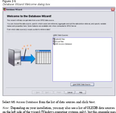
Data from database sources are easily imported using the Database Wizard. Any database that uses ODBC (Open Database Connectivity) drivers can be read directly after the drivers are installed. ODBC drivers for many database formats are supplied on the installation CD. Additional drivers can be obtained from third-party vendors. One of the most common database applications, Microsoft Access, is discussed in this example.
Note: This example is specific to Microsoft Windows and requires an ODBC driver for Access. The steps are similar on other platforms but may require a third-party ODBC driver for Access.
E From the menus choose:
File
Figure 2-5
Database Wizard Welcome dialog box
E SelectMS Access Databasefrom the list of data sources and clickNext.
Figure 2-6
ODBC Driver Login dialog box
E ClickBrowseto navigate to the Access databasefile that you want to open.
E Opendemo.mdb. For more information, seeSample Filesin Appendix A on p. 194.
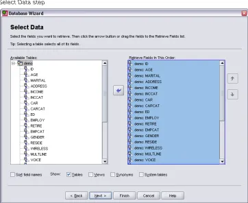
In the next step, you can specify the tables and variables that you want to import.
Figure 2-7 Select Data step
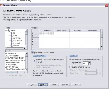
In the next step, you select which records (cases) to import.
Figure 2-8
Limit Retrieved Cases step
If you do not want to import all cases, you can import a subset of cases (for example, males older than 30), or you can import a random sample of cases from the data source. For large data sources, you may want to limit the number of cases to a small, representative sample to reduce the processing time.
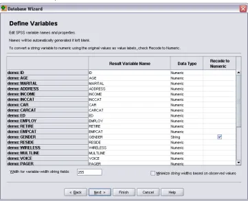
Field names are used to create variable names. If necessary, the names are converted to valid variable names. The originalfield names are preserved as variable labels. You can also change the variable names before importing the database.
Figure 2-9
Define Variables step
E Click theRecode to Numericcell in the Genderfield. This option converts string variables to integer variables and retains the original value as the value label for the new variable.
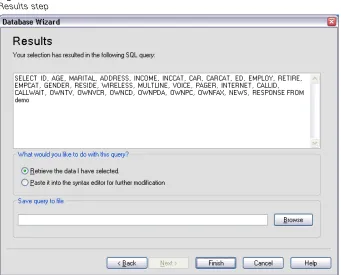
The SQL statement created from your selections in the Database Wizard appears in the Results step. This statement can be executed now or saved to afile for later use.
Figure 2-10 Results step
All of the data in the Access database that you selected to import are now available in the Data Editor.
Figure 2-11
Data imported from an Access database
Reading Data from a Text File
Textfiles are another common source of data. Many spreadsheet programs and databases can save their contents in one of many textfile formats. Comma- or tab-delimitedfiles refer to rows of data that use commas or tabs to indicate each variable. In this example, the data are tab delimited.
E From the menus choose:
File
Read Text Data...
E SelectText (*.txt)as thefile type you want to view.
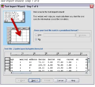
The Text Import Wizard guides you through the process of defining how the specified textfile should be interpreted.
Figure 2-12
Text Import Wizard: Step 1 of 6
E In Step 1, you can choose a predefined format or create a new format in the wizard.
SelectNoto indicate that a new format should be created.
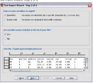
As stated earlier, thisfile uses tab-delimited formatting. Also, the variable names are defined on the top line of thisfile.
Figure 2-13
Text Import Wizard: Step 2 of 6
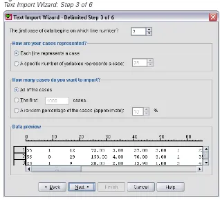
E Type2in the top section of next dialog box to indicate that thefirst row of data starts
on the second line of the textfile.
Figure 2-14
Text Import Wizard: Step 3 of 6
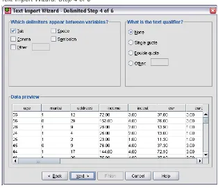
The Data preview in Step 4 provides you with a quick way to ensure that your data are being properly read.
Figure 2-15
Text Import Wizard: Step 4 of 6
Because the variable names may have been truncated tofit formatting requirements, this dialog box gives you the opportunity to edit any undesirable names.
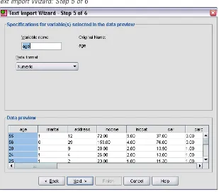
Figure 2-16
Text Import Wizard: Step 5 of 6
Data types can be defined here as well. For example, it’s safe to assume that the income variable is meant to contain a certain dollar amount.
To change a data type:
E Under Data preview, select the variable you want to change, which isIncomein this
E SelectDollarfrom the Data format drop-down list.
Figure 2-17
Change the data type
Figure 2-18
Text Import Wizard: Step 6 of 6
3
Using the Data Editor
The Data Editor displays the contents of the active datafile. The information in the Data Editor consists of variables and cases.
In Data View, columns represent variables, and rows represent cases (observations).
In Variable View, each row is a variable, and each column is an attribute that is associated with that variable.
Variables are used to represent the different types of data that you have compiled. A common analogy is that of a survey. The response to each question on a survey is equivalent to a variable. Variables come in many different types, including numbers, strings, currency, and dates.
Entering Numeric Data
Data can be entered into the Data Editor, which may be useful for small datafiles or for making minor edits to larger datafiles.
E Click theVariable Viewtab at the bottom of the Data Editor window.
You need to define the variables that will be used. In this case, only three variables are needed: age,marital status, andincome.
Figure 3-1
Variable names in Variable View
E In thefirst row of thefirst column, typeage.
E In the second row, typemarital.
E In the third row, typeincome.
New variables are automatically given a Numeric data type.
If you don’t enter variable names, unique names are automatically created. However, these names are not descriptive and are not recommended for large datafiles.
E Click theData Viewtab to continue entering the data.
Begin entering data in thefirst row, starting at thefirst column.
Figure 3-2
Values entered in Data View
E In theagecolumn, type55.
E In themaritalcolumn, type1.
E In theincomecolumn, type72000.
E Move the cursor to the second row of thefirst column to add the next subject’s data.
E In theagecolumn, type53.
E In themaritalcolumn, type0.
E In theincomecolumn, type153000.
Currently, theageandmaritalcolumns display decimal points, even though their values are intended to be integers. To hide the decimal points in these variables:
E In theDecimalscolumn of theagerow, type0to hide the decimal.
E In theDecimalscolumn of themaritalrow, type0to hide the decimal.
Figure 3-3
Updated decimal property for age and marital
Entering String Data
Non-numeric data, such as strings of text, can also be entered into the Data Editor.
E Click theVariable Viewtab at the bottom of the Data Editor window.
E In thefirst cell of thefirst empty row, typesexfor the variable name.
E Click the button on the right side of theTypecell to open the Variable Type dialog box.
Figure 3-4
Button shown in Type cell for sex
E ClickOKto save your selection and return to the Data Editor.
Figure 3-5
Variable Type dialog box
Defining Data
In addition to defining data types, you can also define descriptive variable labels and value labels for variable names and data values. These descriptive labels are used in statistical reports and charts.
Adding Variable Labels
Labels are meant to provide descriptions of variables. These descriptions are often longer versions of variable names. Labels can be up to 255 bytes. These labels are used in your output to identify the different variables.
E Click theVariable Viewtab at the bottom of the Data Editor window. E In theLabelcolumn of theagerow, typeRespondent's Age.
E In theLabelcolumn of themaritalrow, typeMarital Status.
E In theLabelcolumn of thesexrow, typeGender.
Figure 3-6
Variable labels entered in Variable View
Changing Variable Type and Format
TheTypecolumn displays the current data type for each variable. The most common data types are numeric and string, but many other formats are supported. In the current datafile, theincomevariable is defined as a numeric type.
E Click theTypecell for theincomerow, and then click the button on the right side of the
E SelectDollar.
Figure 3-7
Variable Type dialog box
The formatting options for the currently selected data type are displayed.
E For the format of the currency in this example, select$###,###,###.
E ClickOKto save your changes.
Adding Value Labels for Numeric Variables
Value labels provide a method for mapping your variable values to a string label. In this example, there are two acceptable values for themaritalvariable. A value of 0 means that the subject is single, and a value of 1 means that he or she is married.
E Click theValuescell for themaritalrow, and then click the button on the right side of
the cell to open the Value Labels dialog box.
Thevalueis the actual numeric value.
Thevalue labelis the string label that is applied to the specified numeric value.
E TypeSinglein the Labelfield.
E ClickAddto add this label to the list.
Figure 3-8
Value Labels dialog box
E Type1in the Valuefield, and typeMarriedin the Labelfield.
E ClickAdd, and then clickOKto save your changes and return to the Data Editor. These labels can also be displayed in Data View, which can make your data more readable.
E Click theData Viewtab at the bottom of the Data Editor window.
E From the menus choose:
View
Value Labels
If the Value Labels menu item is already active (with a check mark next to it), choosingValue Labelsagain will turnoffthe display of value labels.
Figure 3-9
Value labels displayed in Data View
Adding Value Labels for String Variables
String variables may require value labels as well. For example, your data may use single letters,MorF, to identify the sex of the subject. Value labels can be used to specify thatMstands forMaleandFstands forFemale.
E Click theVariable Viewtab at the bottom of the Data Editor window.
E Click theValuescell in thesexrow, and then click the button on the right side of the
cell to open the Value Labels dialog box.
E ClickAddto add this label to your datafile.
Figure 3-10
Value Labels dialog box
E TypeMin the Valuefield, and typeMalein the Labelfield.
E ClickAdd, and then clickOKto save your changes and return to the Data Editor. Because string values are case sensitive, you should be consistent. A lowercasemis not the same as an uppercaseM.
Using Value Labels for Data Entry
You can use value labels for data entry.
E Click theData Viewtab at the bottom of the Data Editor window. E In thefirst row, select the cell forsex.
E Click the button on the right side of the cell, and then chooseMalefrom the drop-down list.
E Click the button on the right side of the cell, and then chooseFemalefrom the
drop-down list.
Figure 3-11
Using variable labels to select values
Only defined values are listed, which ensures that the entered data are in a format that you expect.
Handling Missing Data
Missing or invalid data are generally too common to ignore. Survey respondents may refuse to answer certain questions, may not know the answer, or may answer in an unexpected format. If you don’tfilter or identify these data, your analysis may not provide accurate results.
Figure 3-12
Missing values displayed as periods
The reason a value is missing may be important to your analysis. For example, you mayfind it useful to distinguish between those respondents who refused to answer a question and those respondents who didn’t answer a question because it was not applicable.
Missing Values for a Numeric Variable
E Click theVariable Viewtab at the bottom of the Data Editor window.
E Click theMissingcell in theagerow, and then click the button on the right side of the
In this dialog box, you can specify up to three distinct missing values, or you can specify a range of values plus one additional discrete value.
Figure 3-13
Missing Values dialog box
E SelectDiscrete missing values.
E Type999in thefirst text box and leave the other two text boxes empty.
E ClickOKto save your changes and return to the Data Editor.
Now that the missing data value has been added, a label can be applied to that value.
E Click theValuescell in theagerow, and then click the button on the right side of the
cell to open the Value Labels dialog box.
E TypeNo Responsein the Labelfield.
Figure 3-14
Value Labels dialog box
E ClickAddto add this label to your datafile.
E ClickOKto save your changes and return to the Data Editor.
Missing Values for a String Variable
Missing values for string variables are handled similarly to the missing values for numeric variables. However, unlike numeric variables, emptyfields in string variables are not designated as system-missing. Rather, they are interpreted as an empty string.
E Click theVariable Viewtab at the bottom of the Data Editor window.
E Click theMissingcell in thesexrow, and then click the button on the right side of the
cell to open the Missing Values dialog box.
E SelectDiscrete missing values.
E TypeNRin thefirst text box.
E ClickOKto save your changes and return to the Data Editor.
Now you can add a label for the missing value.
E Click theValuescell in thesexrow, and then click the button on the right side of the
cell to open the Value Labels dialog box.
E TypeNRin the Valuefield.
E TypeNo Responsein the Labelfield.
Figure 3-15
Value Labels dialog box
E ClickAddto add this label to your project.
E ClickOKto save your changes and return to the Data Editor.
Copying and Pasting Variable Attributes
E In Variable View, typeagewedin thefirst cell of thefirst empty row.
Figure 3-16
agewed variable in Variable View
E In theLabelcolumn, typeAge Married.
E Click theValuescell in theagerow.
E From the menus choose:
Edit Copy
E Click theValuescell in theagewedrow.
E From the menus choose:
Edit Paste
To apply the attribute to multiple variables, simply select multiple target cells (click and drag down the column).
Figure 3-17
Multiple cells selected
When you paste the attribute, it is applied to all of the selected cells.
To copy all attributes from one variable to another variable:
E Click the row number in themaritalrow.
Figure 3-18 Selected row
E From the menus choose:
Edit Copy
E Click the row number of thefirst empty row.
E From the menus choose:
All attributes of themaritalvariable are applied to the new variable.
Figure 3-19
All values pasted into a row
Defining Variable Properties for Categorical Variables
For categorical (nominal, ordinal) data, you can use Define Variable Properties to define value labels and other variable properties. The Define Variable Properties process:
Scans the actual data values and lists all unique data values for each selected variable.
Identifies unlabeled values and provides an “auto-label” feature.
Provides the ability to copy defined value labels from another variable to the selected variable or from the selected variable to additional variables.
E In Data View of the Data Editor, click thefirst data cell for the variableownpc(you
may have to scroll to the right), and then enter99.
E From the menus choose:
Data
Define Variable Properties...
Figure 3-20
Initial Define Variable Properties dialog box
In the initial Define Variable Properties dialog box, you select the nominal or ordinal variables for which you want to define value labels and/or other properties.
E Drag and dropOwns computer [ownpc]throughOwns VCR [ownvcr]into the
Variables to Scan list.
E ClickContinue.
Figure 3-21
Define Variable Properties main dialog box
E In the Scanned Variable List, selectownpc.
The current level of measurement for the selected variable is scale. You can change the measurement level by selecting a level from the drop-down list, or you can let Define Variable Properties suggest a measurement level.
E ClickSuggest.
Figure 3-22
Suggest Measurement Level dialog box
Because the variable doesn’t have very many different values and all of the scanned cases contain integer values, the proper measurement level is probably ordinal or nominal.
E SelectOrdinal, and then clickContinue.
The measurement level for the selected variable is now ordinal.
The Value Label grid displays all of the unique data values for the selected variable, any defined value labels for these values, and the number of times (count) that each value occurs in the scanned cases.
Scanned Variable List also indicates that the selected variable has at least one observed value without a defined value label.
E In theLabelcolumn for the value of 99, enterNo answer.
E Check the box in theMissingcolumn for the value 99 to identify the value 99 as
user-missing.
Data values that are specified as user-missing areflagged for special treatment and are excluded from most calculations.
Figure 3-23
New variable properties defined for ownpc
Before we complete the job of modifying the variable properties forownpc, let’s apply the same measurement level, value labels, and missing values definitions to the other variables in the list.
Figure 3-24
Apply Labels and Level dialog box
E In the Apply Labels and Level dialog box, select all of the variables in the list, and
If you select any other variable in the Scanned Variable List of the Define Variable Properties main dialog box now, you’ll see that they are all ordinal variables, with a value of 99 defined as user-missing and a value label ofNo answer.
Figure 3-25
New variable properties defined for ownfax
4
Working with Multiple Data
Sources
Starting with version 14.0, multiple data sources can be open at the same time, making it easier to:
Switch back and forth between data sources.
Compare the contents of different data sources.
Copy and paste data between data sources.
Create multiple subsets of cases and/or variables for analysis.
Merge multiple data sources from various data formats (for example, spreadsheet, database, text data) without saving each data sourcefirst.
Basic Handling of Multiple Data Sources
Figure 4-1Two data sources open at same time
By default, each data source that you open is displayed in a new Data Editor window.
Any previously open data sources remain open and available for further use.
When youfirst open a data source, it automatically becomes theactive dataset.
Only the variables in the active dataset are available for analysis.
Figure 4-2
Variable list containing variables in the active dataset
You cannot change the active dataset when any dialog box that accesses the data is open (including all dialog boxes that display variable lists).
Working with Multiple Datasets in Command Syntax
If you use command syntax to open data sources (for example,GET FILE,GET DATA), you need to use theDATASET NAMEcommand to name each dataset explicitly in order to have more than one data source open at the same time.
When working with command syntax, the active dataset name is displayed on the toolbar of the syntax window. All of the following actions can change the active dataset:
Use theDATASET ACTIVATEcommand.
Click anywhere in the Data Editor window of a dataset.
Select a dataset name from the toolbar in the syntax window.
Figure 4-3
Open datasets displayed on syntax window toolbar
Copying and Pasting Information between Datasets
You can copy both data and variable definition attributes from one dataset to another dataset in basically the same way that you copy and paste information within a single datafile.
Copying and pasting selected data cells in Data View pastes only the data values, with no variable definition attributes.
Copying and pasting variable definition attributes or entire variables in Variable View pastes the selected attributes (or the entire variable definition) but does not paste any data values.
Renaming Datasets
When you open a data source through the menus and dialog boxes, each data source is automatically assigned a dataset name ofDataSetn, wherenis a sequential integer value, and when you open a data source using command syntax, no dataset name is assigned unless you explicitly specify one withDATASET NAME. To provide more descriptive dataset names:
E From the menus in the Data Editor window for the dataset whose name you want
to change choose:
File
Rename Dataset...
E Enter a new dataset name that conforms to variable naming rules.
Suppressing Multiple Datasets
If you prefer to have only one dataset available at a time and want to suppress the multiple dataset feature:
E From the menus choose:
Edit Options...
E Click theGeneraltab.
5
Examining Summary Statistics for
Individual Variables
This chapter discusses simple summary measures and how the level of measurement of a variable influences the types of statistics that should be used. We will use the datafile
demo.sav. For more information, seeSample Filesin Appendix A on p. 194.
Level of Measurement
Different summary measures are appropriate for different types of data, depending on the level of measurement:
Categorical.Data with a limited number of distinct values or categories (for example, gender or marital status). Also referred to asqualitative data. Categorical variables can be string (alphanumeric) data or numeric variables that use numeric codes to represent categories (for example, 0 =Unmarriedand 1 =Married). There are two basic types of categorical data:
Nominal.Categorical data where there is no inherent order to the categories. For example, a job category ofsalesis not higher or lower than a job category of
marketingorresearch.
Ordinal. Categorical data where there is a meaningful order of categories, but there is not a measurable distance between categories. For example, there is an order to the valueshigh,medium, andlow, but the “distance” between the values cannot be calculated.
Scale.Data measured on an interval or ratio scale, where the data values indicate both the order of values and the distance between values. For example, a salary of $72,195 is higher than a salary of $52,398, and the distance between the two values is $19,797. Also referred to asquantitativeorcontinuous data.
Summary Measures for Categorical Data
For categorical data, the most typical summary measure is the number or percentage of cases in each category. Themodeis the category with the greatest number of cases. For ordinal data, themedian(the value at which half of the cases fall above and below) may also be a useful summary measure if there is a large number of categories.
The Frequencies procedure produces frequency tables that display both the number and percentage of cases for each observed value of a variable.
E From the menus choose:
Analyze
Descriptive Statistics Frequencies...
E SelectOwns PDA [ownpda]andOwns TV [owntv]and move them into the Variable(s)
list.
Figure 5-1
Categorical variables selected for analysis
Figure 5-2 Frequency tables
The frequency tables are displayed in the Viewer window. The frequency tables reveal that only 20.4% of the people own PDAs, but almost everybody owns a TV (99.0%). These might not be interesting revelations, although it might be interesting tofind out more about the small group of people who do not own televisions.
Charts for Categorical Data
You can graphically display the information in a frequency table with a bar chart or pie chart.
You can use the Dialog Recall button on the toolbar to quickly return to recently used procedures.
Figure 5-3
Dialog Recall button
E ClickCharts.
E SelectBar chartsand then clickContinue.
Figure 5-4
Frequencies Charts dialog box
Figure 5-5 Bar chart
In addition to the frequency tables, the same information is now displayed in the form of bar charts, making it easy to see that most people do not own PDAs but almost everyone owns a TV.
Summary Measures for Scale Variables
There are many summary measures available for scale variables, including:
Measures of central tendency. The most common measures of central tendency are themean(arithmetic average) andmedian(value at which half the cases fall above and below).
Measures of dispersion.Statistics that measure the amount of variation or spread in the data include the standard deviation, minimum, and maximum.
E Open the Frequencies dialog box again.
E SelectHousehold income in thousands [income]and move it into the Variable(s) list.
Figure 5-6
Scale variable selected for analysis
E SelectMean,Median,Std. deviation,Minimum, andMaximum.
Figure 5-7
Frequencies Statistics dialog box
E ClickContinue.
E DeselectDisplay frequency tablesin the main dialog box. (Frequency tables are usually
not useful for scale variables since there may be almost as many distinct values as there are cases in the datafile.)
The Frequencies Statistics table is displayed in the Viewer window.
Figure 5-8
Frequencies Statistics table
In this example, there is a large difference between the mean and the median. The mean is almost 25,000 greater than the median, indicating that the values are not normally distributed. You can visually check the distribution with a histogram.
Histograms for Scale Variables
E Open the Frequencies dialog box again.
E SelectHistogramsandWith normal curve.
Figure 5-9
Frequencies Charts dialog box
Figure 5-10 Histogram
6
Creating and Editing Charts
You can create and edit a wide variety of chart types. In this chapter, we will create and edit bar charts. You can apply the principles to any chart type.
Chart Creation Basics
To demonstrate the basics of chart creation, we will create a bar chart of mean income for different levels of job satisfaction. This example uses the datafiledemo.sav. For more information, seeSample Filesin Appendix A on p. 194.
E From the menus choose:
Graphs
Chart Builder...
The Chart Builder dialog box is an interactive window that allows you to preview how a chart will look while you build it.
Figure 6-1
Chart Builder dialog box
Using the Chart Builder Gallery
The Gallery includes many different predefined charts, which are organized by chart type. The Basic Elements tab also provides basic elements (such as axes and graphic elements) for creating charts from scratch, but it’s easier to use the Gallery.
E ClickBarif it is not selected.
E Drag the icon for the simple bar chart onto the “canvas,” which is the large area above
the Gallery. The Chart Builder displays a preview of the chart on the canvas. Note that the data used to draw the chart are not your actual data. They are example data.
Figure 6-2
Defining Variables and Statistics
Although there is a chart on the canvas, it is not complete because there are no variables or statistics to control how tall the bars are and to specify which variable category corresponds to each bar. You can’t have a chart without variables and statistics. You add variables by dragging them from the Variables list, which is located to the left of the canvas.
A variable’s measurement level is important in the Chart Builder. You are going to use theJob satisfactionvariable on thexaxis. However, the icon (which looks like a ruler) next to the variable indicates that its measurement level is defined as scale. To create the correct chart, you must use a categorical measurement level. Instead of going back and changing the measurement level in the Variable View, you can change the measurement level temporarily in the Chart Builder.
E Right-clickJob satisfactionin the Variables list and chooseOrdinal. Ordinal is an
E Now dragJob satisfactionfrom the Variables list to thexaxis drop zone.
Figure 6-3
Job satisfaction in x axis drop zone
Theyaxis drop zone defaults to theCountstatistic. If you want to use another statistic (such as percentage or mean), you can easily change it. You will not use either of these statistics in this example, but we will review the process in case you need to change this statistic at another time.
Figure 6-4
Element Properties window
The Element Properties window allows you to change the properties of the various chart elements. These elements include the graphic elements (such as the bars in the bar chart) and the axes on the chart. Select one of the elements in the Edit Properties of list to change the properties associated with that element. Also note the redX
The Statistic drop-down list shows the specific statistics that are available. The same statistics are usually available for every chart type. Be aware that some statistics require that theyaxis drop zone contains a variable.
E Return to the Chart Builder dialog box and dragHousehold income in thousandsfrom
the Variables list to theyaxis drop zone. Because the variable on theyaxis is scalar and thexaxis variable is categorical (ordinal is a type of categorical measurement level), theyaxis drop zone defaults to theMeanstatistic. These are the variables and statistics you want, so there is no need to change the element properties.
Adding Text
You can also add titles and footnotes to the chart.
E Click theTitles/Footnotestab.
Figure 6-5
Title 1 displayed on canvas
The title appears on the canvas with the labelT1.
E In the Element Properties window, selectTitle 1in the Edit Properties of list. E In the Content text box, typeIncome by Job Satisfaction. This is the text that the
title will display.
Creating the Chart
E ClickOKto create the bar chart.
Figure 6-6 Bar chart
The bar chart reveals that respondents who are more satisfied with their jobs tend to have higher household incomes.
Chart Editing Basics
You can edit charts in a variety of ways. For the sample bar chart that you created, you will:
Format numbers in tick labels.
Edit text.
Display data value labels.
Use chart templates.
To edit the chart, open it in the Chart Editor.
E Double-click the bar chart to open it in the Chart Editor.
Figure 6-7
Bar chart in the Chart Editor
Selecting Chart Elements
To edit a chart element, youfirst select it.
There are general rules for selecting elements in simple charts:
When no graphic elements are selected, click any graphic element to select all graphic elements.
When all graphic elements are selected, click a graphic element to select only that graphic element. You can select a different graphic element by clicking it. To select multiple graphic elements, click each element while pressing the Ctrl key.
E To deselect all elements, press the Esc key.
E Click any bar to select all of the bars again.
Using the Properties Window
E From the Chart Editor menus choose:
This opens the Properties window, showing the tabs that apply to the bars you selected. These tabs change depending on what chart element you select in the Chart Editor. For example, if you had selected a text frame instead of bars, different tabs would appear in the Properties window. You will use these tabs to do most chart editing.
Figure 6-8 Properties window
Changing Bar Colors
First, you will change the color of the bars. You specify color attributes of graphic elements (excluding lines and markers) on the Fill & Border tab.
E Click the swatch next to Fill to indicate that you want to change thefill color of the
bars. The numbers below the swatch specify the red, green, and blue settings for the current color.
E Click the light blue color, which is second from the left in the second row from the
bottom.
Figure 6-9 Fill & Border tab
The bars in the chart are now light blue.
Figure 6-10
Edited bar chart showing blue bars
Formatting Numbers in Tick Labels
Notice that the numbers on theyaxis are scaled in thousands. To make the chart more attractive and easier to interpret, we will change the number format in the tick labels and then edit the axis title appropriately.
E Select theyaxis tick labels by clicking any one of them.
E To reopen the Properties window (if you closed it previously), from the menus choose:
Edit Properties
Note: From here on, we assume that the Properties window is open. If you have closed the Properties window, follow the previous step to reopen it. You can also use the keyboard shortcut Ctrl+T to reopen the window.
E You do not want the tick labels to display decimal places, so type0in the Decimal
Places text box.
E Type0.001in the Scaling Factor text box. The scaling factor is the number by which
the Chart Editor divides the displayed number. Because0.001is a fraction, dividing by it willincreasethe numbers in the tick labels by 1,000. Thus, the numbers will no longer be in thousands; they will be unscaled.
E SelectDisplay Digit Grouping. Digit grouping uses a character (specified by your computer’s locale) to mark each thousandth place in the number.
Figure 6-11 Number Format tab
The tick labels reflect the new number formatting: There are no decimal places, the numbers are no longer scaled, and each thousandth place is specified with a character.
Figure 6-12
Edited bar chart showing new number format
Editing Text
Now that you have changed the number format of the tick labels, the axis title is no longer accurate. Next, you will change the axis title to reflect the new number format.
Note: You do not need to open the Properties window to edit text. You can edit text directly on the chart.
E Click theyaxis title to select it.
E Click the axis title again to start edit mode. While in edit mode, the Chart Editor
E Delete the following text:
in thousands
E Press Enter to exit edit mode and update the axis title. The axis title now accurately
describes the contents of the tick labels.
Figure 6-13
Bar chart showing edited y axis title
Displaying Data Value Labels
Another common task is to show the exact values associated with the graphic elements (which are bars in this example). These values are displayed in data labels.
E From the Chart Editor menus choose:
Elements
Figure 6-14
Bar chart showing data value labels
Each bar in the chart now displays the exact mean household income. Notice that the units are in thousands, so you could use the Number Format tab again to change the scaling factor.
Using Templates
If you make a number of routine changes to your charts, you can use a chart template to reduce the time needed to create and edit charts. A chart template saves the attributes of a specific chart. You can then apply the template when creating or editing a chart.
We will save the current chart as a template and then apply that template while creating a new chart.
E From the menus choose:
File
Save Chart Template...
If you expand any of the items in the tree view, you can see which specific attributes can be saved with the chart. For example, if you expand theScale axesportion of the tree, you can see all of the attributes of data value labels that the template will include. You can select any attribute to include it in the template.
E SelectAll settingsto include all of the available chart attributes in the template. You can also enter a description of the template. This description will be visible when you apply the template.
Figure 6-15
Save Chart Template dialog box
E ClickContinue.
E When you arefinished, clickSave.
You can apply the template when you create a chart or in the Chart Editor. In the following example, we will apply it while creating a chart.
E Close the Chart Editor. The updated bar chart is shown in the Viewer.
Figure 6-16
Upda