ECONOMIC ORDER QUANTITY MODEL UNDER TRAD

240

REVISTA INVESTIGACION OPERACIONAL VOL. 36, NO. 3, 240-248, 2015

ECONOMIC ORDER QUANTITY MODEL UNDER

TRADE CREDIT AND CUSTOMER RETURNS FOR

PRICE-SENSITIVE QUADRATIC DEMAND

Nita H. Shah*1_{, Mrudul Y. Jani** and Digeshkumar B. Shah***}

*_{Department of Mathematics, Gujarat University, Ahmedabad-380009, Gujarat,}

**_{Department of Mathematics, Parul Institute of Engg. and Technology, Vadodara-391760, Gujarat} ***_{Department of Mathematics, L.D. College of Engineering, Ahmedabad-380009, Gujarat}

ABSTRACT

This article focuses on an inventory model in which a supplier gives credit for a prior mutually agreed fixed period to a retailer. In this model, the simultaneous determination of price and inventory replenishment when customers return product to the firm are given due importance. Price-sensitive quadratic demand is debated here; which is appropriate for the products for which demand increases initially and after sometime it starts to decrease. Lastly, retailer’s total profit is maximized with respect to selling price and cycle time. Numerical examples are given to authenticate the model. Through sensitivity analysis significant inventory parameters are filtered. Graphical outcomes, in two and three dimensions, are presented and managerial decisions are provided with multiple options.

RESUMEN

Este artículo se centra en un modelo de inventario en el que un proveedor le da crédito para un mutuo acuerdo previo período fijo que un minorista. En este modelo, la determinación simultánea de precio y reposición de inventarios cuando los clientes devuelven el producto a la empresa dada la debida importancia. La ecuación cuadrática precio-sensible es debatida aquí; que es el tiempo apropiado para los productos cuya demanda aumenta inicialmente y después de un tiempo, comienza a disminuir. Por último, el beneficio minorista total se maximiza con respecto al precio de venta y al tiempo de ciclo. Ejemplos numéricos son dadas para autenticar el modelo. Mediante análisis de sensibilidad significativa los parámetros de inventario son filtrados. Los resultados gráficos, en dos y tres dimensiones, se presentan y las decisiones de gestión se proporcionan con múltiples opciones.

KEYWORDS Inventory model, credit period, customer returns, quadratic demand, selling price, cycle time

MSC: 90B05

1. INTRODUCTION

Haris-Wilson’s economic order quantity model is based on the supposition that a seller uses cash-on delivery policy. But In the market, if the buyer has an option to pay later on without interest charges then he gets attracted to buy. And this may be proved to be an excellent strategy in today’s cutthroat scenario. During this allowable period, the retailer can earn interest on sold items. Goyal (1985) prepared decision policy by incorporating concept of allowable delay in payments to settle the accounts due against purchases in the classical EOQ model. Thereafter, credit period and its variants were given by several researchers. Shah et al. (2010) gave review article on inventory modeling with trade credits. Jaggi et al. (2008) analyzed retailer’s optimal policy with credit linked demand under permissible delay in payments. Jamal et al. (2000) modelled optimal payment time for retailer under permissible delay by supplier. Chang et al. (2001) incorporated linear trend demand in inventory model under the condition of permissible delay in payment. Lou and Wang (2013)

studied the seller’s decision about setting delay payment period. They used deterministic constant demand. Almost all the researchers concluded that the length of trade credit increases the demand rate.

In supply chain management returns of product from customers to retailers is a major problem and return strategy can be considered as an essential competition. Chen and Bell (2009) discussed how the company should change price and inventory replenishment in order to ease the negative effects of returns from customers. Ghoreishi et al. (2012) studied the effect of inflation and customer returns on the joint pricing and inventory control for deteriorating items. They assumed that the customer returns increase with both the quantity sold and

the product price. Hu and Li (2012) integrated a retailer’s return policy and a supplier’s buyback policy within a modeling framework. They showed that supplier's best preference is to provide buyback policy and the

retailer’s optimal response is to set refund price to be the same as supplier’s buyback price. He et al. (2006) developed a model to determine optimal return policies for single period products based on unsure market demands and in the presence of risk preferences. Pasternach (1985) proved that a pricing and return policy in

1

Corresponding Author: 1_{Prof Nita H. Shah}

241

which a manufacturer offers retailers a partial credit for all unsold goods can achieve channel coordination in a multi-retailer environment.

In above cited articles, mostly all the researchers considered demand rate to be constant. However, the market survey says that the demand hardly remains constant. In this paper, we considered demand to be price-sensitive time quadratic. Quadratic demand initially increases with time for some time and then decreases. In the model supplier gives credit period to his customers for payment. Also customers return products back to the company. The focus is to maximize the total profit per unit time for the retailer. Numerical examples and graphical analysis are provided. At last, we take sensitivity analysis to study the consequences on optimal solution with respect to one inventory parameter at a time. For the retailer, managerial insights are furnished.

2. NOTATIONS AND ASSUMPTIONS

h

Inventory holding cost (excluding interest charges) per unit per unit time

M

Credit period offered by the supplier to the retailer

e

I

Interest earned per $ per year

c

I

Interest charged per $ for unsold stock per annum by the supplier

Note:

I

_c



I

_e

 

R P,t

Price sensitive time dependent demand

 

I t

Inventory level at any instant of time t ,

0

 

t

T

T

Cycle time ( a decision variable)

Q

Ordering quantity per cycle

4. Shortages are not allowed. Lead-time is zero or negligible. 5. The initial and final inventory levels both are zero.

6. The retailer generates revenue by selling items and earns interest during

 

0

,

M

with rate

I

_e.

242 3. MATHEMATICAL MODEL

We analyse one inventory cycle. The rate of change of inventory level at any instant of time t is governed by the differential equation

 

_{ }

_{, , 0}

dI t

R P t

t

T

dt

 

 

(1)

Using initial condition

I T

 



0

, the solution of differential equation (1) is given by

 

1

2 2

1

3 3

(

)

(

) , 0

2

3

I t



aP



_



T

 

t

b T



t



c T



t



_

 

t

T





(2)

Consequently, the ordering quantity for the retailer is

 

1

2

1

3

0

2

3

Q



I



aP





_

T



bT



cT



_





(3)

The cost components per cycle for the retailer are as follows.

Sales revenue;

 

Now, depending upon the credit period and cycle time we have two different cases:

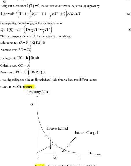
Case - 1:

M



T

(Figure 1)

Figure 1 Interest earned and charged when

M



T

In this case, the allowable credit period is less than or equal to the cycle time. During

 

0, M

the buyer earns

interest at the rate e

I

on the generated income. The interest earned per unit time is

243

Hence, the total profit per unit time for retailer is

 





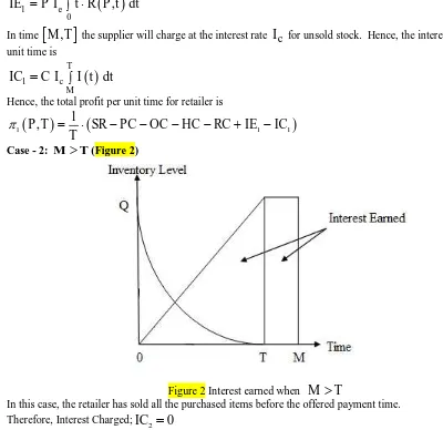
In this case, the retailer has sold all the purchased items before the offered payment time. Therefore, Interest Charged;

IC

₂



0

Hence, the total profit per unit time for retailer is

 





Therefore, the total profit of the retailer can be given by

 

1

 

_{ }

Now, the necessary conditions to make total profit maximum are

 

₀

Here, we adopt following algorithm for the solution.

Step 1: Allocate hypothetical values to the inventory parameters.

Step 2: Solve equations in (5) simultaneously by mathematical software Maple XIV. Step 3: Check second order (sufficiency) conditions

244

Step 4: Compute profit;



 

P ,T

per unit time from equation (4) and ordering quantity

Q

from equation (3).

The aim is to make total profit per unit time maximum with respect to selling price and cycle time. Now, we examine the working of the model with numerical values for the inventory parameters.

4. NUMERICAL EXAMPLES AND SENSITIVITY ANALYSIS

Example:1 Taking

A



$

200

per order,

C



$

20

per unit,

h



$

4

/unit/year,

a



10000

units,

b



5%

,

10%



c

,





1.2

,





0.1

,





0.4

,

I

_e



9%

/

$

/year

,

I

_c



15

%

/

$

/year

and

year

365

30



M

.

The optimal cycle time

 

T

is 0.72 years, optimal retail price

 

P

is $47.25 and corresponding profit is

$814.187.Clearly, here

M



T

.The retailer’s purchase is 70.63 units. The concavity of the profit function is demonstrated in figure 3.

Figure 3 Concavity of total profit w. r. t. cycle time

 

T

and retail price

 

P

for

M



T

Example:2 Taking

A



$ 100

per order,

C



$

20

per unit,

h



$

4

/unit/year,

a



1000000

units,

5%



b

,

c



20%

,





1.2

,





0.1

,





0.4

,

I

e



9%

/

$

/year

,

I

c



15

%

/

$

/year

and

year

365

30



M

. The optimal cycle time

 

T

is 0.071 years, optimal retail price

 

P

is $115.88 and

245

Figure 4 Concavity of total profit w. r. t. cycle time

 

T

and retail price

 

P

for

M



T

In this case, retailer is enjoying whole benefit in supply chain and supplier suffers a lot. So we don’t consider such a case.

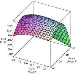
Example: 3 Taking

A



$

200

per order,

C



$

20

per unit,

h



$

4

/unit/year,

a



10000

units,

5%



b

,

c



10%

,





1.2

,





0.1

,





0.4

,

I

_c



15

%

/

$

/year

and. The optimal cycle time

 

T

is 0.72 years, optimal retail price

 

P

is $47.46 and corresponding profit is $789.519. Clearly, here,

M



0

.

The retailer’s purchase is 70.51 units. The concavity of the profit function is demonstrated in figure 5.

246

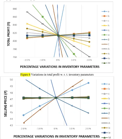
Now, for example 1, we examine the effects of various inventory parameters on total profit, decision variables selling price

 

P

and cycle time

 

T

by varying them as -20%, -10%, 10% and 20%.

Figure 6 Variations in total profit w. r. t. inventory parameters

247

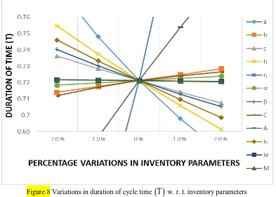
Figure 8 Variations in duration of cycle time

 

T

w. r. t. inventory parameters The observations from the above sensitivity analyses (Figures. 6-8) are as follows.

From Figure. 6, it is observed that scaled demand has huge positive impact on profit whereas linear rate of change of demand

 

b

increases profit marginally. If holding cost increases then obviously profit decreases.

Mark up for trade credit has extremely large negative impact on profit. Purchase cost again obviously decreases profit rapidly. By increasing quadratic rate of change of demand

 

c

, ordering cost

 

A

and interest charged for

unsold stock by the supplier

 

I

_c total profit gets decreased slightly.

From Figure. 7, it is evident that selling price has positive effect of scale demand

 

a

, linear rate of change of

demand

 

b

, ordering cost

 

A

, purchase cost

 

C

, holding cost

 

h

and interest charged for unsold stock by

the supplier

 

I

_c , whereas selling price has negative effect of quadratic rate of change of demand

 

c

, mark up

for trade credit

 



, interest earned

 

I

_e and credit period offered by supplier to retailer

 

M

.

From Figure. 8, we can say that Cycle time has positive effect of linear rate of change of demand

 

b

, ordering

cost

 

A

, purchase cost

 

C

and mark up for trade credit

 



, while cycle time has negative effect of scale

demand

 

a

, quadratic rate of change of demand

 

c

, holding cost

 

h

, credit period offered by supplier to

retailer

 

M

, interest earned

 

I

_e and interest charged for unsold stock by the supplier

 

I

_c .

5. CONCLUSIONS

To offer credit period to the customers is the best promotional tool in the business market. In this article, we have studied an inventory model in which supplier offers credit period to the retailer for the products purchased. In the model, we have assumed that customers return products during cycle time, which is a crucial situation in the competitive market. The model deals with price – sensitive quadratic demand. Quadratic demand can be seen when products are in demand for some time and after that demand decreases gradually for that products for several reasons. The non-linear profit function is obtained. The necessary conditions are expressed to get optimal solution based on the facts. We maximized the retailer’s total profit for retail price and cycle time. Numerical examples and sensitivity analysis are provided to take beneficial decisions for the managers.

For future research, this concept can be extended for stochastic demand and fuzzy demand. One can think of allowing shortages. Also one can add deterioration of inventory products.

248

RECEIVED DECEMBER, 2014 REVISED FEBRUARY, 2015 REFERENCES

[1] CHAN, J. and BELL, P. C., (2009): The impact of customer returns on pricing and order decisions. European Journal of Operational Research, 195 (1), 280-295.

[2] CHANG, H. J., HUNG, C. H. and DYE, C. Y., (2001): An inventory model for deteriorating items with linear trend demand under the condition of permissible delay in payments. Production Planning and Control, 12 (3), 274-282.

[3] GHOREISHI, M., KHAMESEH, A. A. and MIRZAZADEH, A., (2013): Joint optimal pricing and inventory control for deteriorating items under inflation and customer returns. Journal of Industrial Engineering, Volume 2013 (2013), Article ID 709083. http://dx.doi.org/10.1155/2013/709083.

[4] GHOREISHI, M., MIRZAZADEH, A., KAMALABADI, I. N., (2014): Optimal pricing and lot-sizing policies for an economic production quantity model with non-instantaneous deteriorating items, permissible delay in payments, customer returns and inflation. Proceedings of the Institution of Mechanical Engineers, Part B: Journal of Engineering Manufacture. DOI: 10.1177/0954405414522215.

[5] GOYAL, S. K., (1985): Economic order quantity under conditions of permissible delay in payments. Journal of the Operational Research Society, 36, 335-338.

[6] HE, J., CHIN, K. S., YANG, J. B. and ZHU, D. L., (2006): Return policy model of supply chain management for single-period products. Journal of Optimization Theory and Applications, 129 (2), 293-308.

[7] HU, W. and LI, J., (2012): How to implement return policies in a two-echelon supply chain? Discrete Dynamics in Nature and Society, Article ID 453193. http://dx.doi.org/10.1155/2012/453193.

[8] JAGGI, C. K., GOYAL, S. K. and GOEL, S. K., (2008): Retailer’s optimal replenishment decisions with credit-linked demand under permissible delay in payments. European Journal of Operational Research, 190, 130-135.

[9] JAMAL, A. M. M., SARKER, B. R. and WANG, S., (2000): Optimal payment time for a retailer under permitted delay of payment by the wholesaler. International Journal of Production Economics, 66 , 59–66. [10] LOU, K. R. and WANG, W.C., (2013): Optimal trade credit and order quantity when trade credit impacts on both demand rate and default risk. Journal of the Operational Research Society, 64, 1551-1556. [11] PASTERNACK, B. A., (1985): Optimal pricing and return policies for perishable commodities. Marketing Science, 4, 166-176.