Chapter 02.02 Differentiation of Continuous Functions

02.01.1

Chapter 02.02

Differentiation of Continuous Functions

After reading this chapter, you should be able to:

1. derive formulas for approximating the first derivative of a function, 2. derive formulas for approximating derivatives from Taylor series, 3. derive finite difference approximations for higher order derivatives, and 4. use the developed formulas in examples to find derivatives of a function.

The derivative of a function at x is defined as

( )

(

) ( )

x x f x x f x

f

x ∆

− ∆ + =

′

→ ∆lim0

To be able to find a derivative numerically, one could make ∆x finite to give,

( )

(

) ( )

x x f x x f x f

∆ − ∆ + ≈

′ .

Knowing the value of x at which you want to find the derivative of f

( )

x , we choose a value of ∆x to find the value of f′

( )

x . To estimate the value of f′

( )

x , three such approximations are suggested as follows.

Forward Difference Approximation of the First Derivative

From differential calculus, we know

( )

(

) ( )

x x f x x f x

f

x ∆

− ∆ + =

′

→ ∆lim0

For a finite ∆x,

( )

(

) ( )

x x f x x f x f

∆ − ∆ + ≈ ′

The above is the forward divided difference approximation of the first derivative. It is called forward because you are taking a point ahead of x. To find the value of f′

( )

x at x= x_i, we may choose another point ∆x ahead as x= x_i+1. This gives

( )

( )

( )

x x f x f x

f i i

i _∆

− ≈

( )

( )

i i

i i

x x

x f x f

− − =

+ +

1 1

where

i i x x

x= −

∆ ₊₁

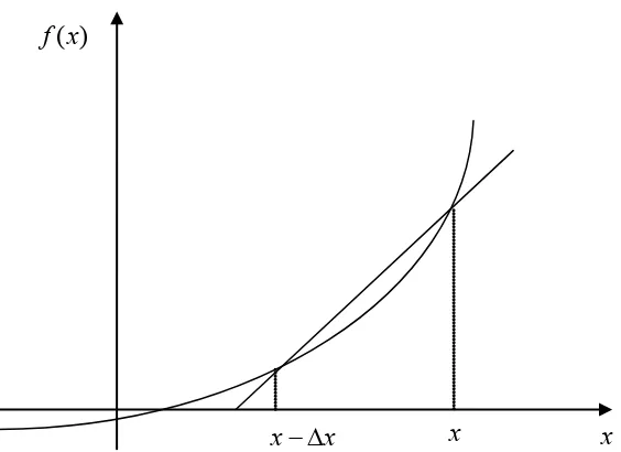
Figure 1 Graphical representation of forward difference approximation of first derivative.

Example 1

The velocity of a rocket is given by

( )

9.8 ,0 30

2100 10

14

10 14 ln

2000 ₄

4

≤ ≤ −

   

 

− ×

×

= t t

t t

ν

where ν is given in m/s and t is given in seconds. At t =16s,

a) use the forward difference approximation of the first derivative of ν

( )

t to calculate the acceleration. Use a step size of ∆t=2s.

b) find the exact value of the acceleration of the rocket. c) calculate the absolute relative true error for part (b).

Solution

(a)

( ) ( ) ( )

t

t t

t

a i i

i _∆

− ≈ν +1 ν

16 = i t

2 Δt =

t t t_i+1 = _i +Δ

2 16+

=

=18 ) (x f

x x+∆

( ) ( ) ( )

(b) The exact value of a

( )

16 can be calculated by differentiating

( )

t

Knowing that

( )

(c) The absolute relative true error is

100 674

. 29

474 . 30 674 . 29

× −

=

=2.6967%

Backward Difference Approximation of the First Derivative

We know

( )

(

) ( )

x x f x x f x

f

x ∆

− ∆ + =

′

→ ∆lim0

For a finite ∆x,

( )

(

) ( )

x x f x x f x f

∆ − ∆ + ≈ ′

If ∆x is chosen as a negative number,

( )

(

) ( )

x x f x x f x f

∆ − ∆ + ≈ ′

( ) (

)

x

x x f x f

Δ Δ − − =

This is a backward difference approximation as you are taking a point backward from x. To find the value of f′

( )

x at x= x_i, we may choose another point ∆x behind as x= x_i−1. This gives

( )

( ) ( )

x x f x f x

f i i

i _∆

− ≈

′ −1

( ) ( )

1 1

− −

− − =

i i

i i

x x

x f x f

where

1

Figure 2 Graphical representation of backward difference approximation of first derivative.

Example 2

The velocity of a rocket is given by

( )

9.8 ,0 30

2100 10

14

10 14 ln

2000 ₄

4

≤ ≤ −

   

 

− ×

×

= t t

t t

ν

(a) Use the backward difference approximation of the first derivative of ν

( )

t to calculate the acceleration at t=16s. Use a step size of ∆t=2s.

(b) Find the absolute relative true error for part (a).

Solution

( ) ( ) ( )

t

t t t

a i i

∆ −

≈ν ν −1

16 = i t

2 Δt =

t t

t_i−1 = _i −Δ =16−2 = 14

( ) ( ) ( )

2

14 16

16 ≈ν −ν a

( )

_{( )}

9.8

( )

16

16 2100 10

14

10 14 ln

2000

16 ₄

4

−    

 

− ×

× =

ν

=392.07m/s

( )

_{( )}

9.8

( )

14

14 2100 10

14

10 14 ln

2000

14 ₄

4

−    

 

− ×

× =

ν

) (x f

x x

=334.24m/s

( ) ( ) ( )

2

14 16

16 ≈ν −ν a

2

24 . 334 07 .

392 −

=

2

m/s 915 . 28

=

(b) The exact value of the acceleration at t=16s from Example 1 is

( )

2

m/s 674 . 29 16 = a

The absolute relative true error for the answer in part (a) is

100 674

. 29

915 . 28 674 .

29 − _×

= ∈_t

=2.5584%

Forward Difference Approximation from Taylor Series

Taylor’s theorem says that if you know the value of a function f(x) at a point x_i and all its

derivatives at that point, provided the derivatives are continuous between x_i and x_i+1, then

( )

₊ =

( )

+ ′

( )(

₊ −

)

+ ′′

( )(

₊ −

)

2+

1 1

1

!

2 i i

i i

i i i

i x x

x f x x x f x f x f

Substituting for convenience Δx= x_i+1−x_i

( )

₊ =

( )

+ ′

( )

+ ′′

( )( )

2+

1 Δ

! 2 Δx f x x x

f x f x

f i

i i

i

( )

( ) ( )

− ′′

( )( )

∆ +

∆ − =

′ + f x _x

x x f x f x

f i i i

i

! 2

1

( )

( ) ( )

O

( )

x x

x f x f x

f i i

i _∆ + ∆

− =

′ +1

The O

( )

∆x term shows that the error in the approximation is of the order of ∆x.

Can you now derive from the Taylor series the formula for the backward divided difference approximation of the first derivative?

As you can see, both forward and backward divided difference approximations of the first derivative are accurate on the order of O

( )

∆x . Can we get better approximations? Yes, another method to approximate the first derivative is called the central difference approximation of the first derivative.

From the Taylor series

( )

₊ =

( )

+ ′

( )

+ ′′

( )( )

2 + ′′′

( )( )

3 +

1 Δ

! 3 Δ

! 2

Δx f x x f x x x

f x f x

f i i

i i

i (1)

and

( )

₋ =

( )

− ′

( )

+ ′′

( )( )

2 − ′′′

( )( )

3 +

1 Δ

! 3 Δ

! 2

Δx f x x f x x x

f x f x

f _{i i i} i i (2)

( ) ( )

₊ − ₋ = ′

( )(

)

+ ′′′

( )( )

3+

1

1 Δ

! 3 2 Δ

2 x f x x

x f x f x

f i

i i

i

( )

( ) ( )

− ′′′

( )( )

∆ +

∆ − =

′ +1 −1 2

! 3

2 x

x f x

x f x f x

f i i i

i

( ) ( )

_{1 1}

_{( )}

2

2 x O x

x f x

f _{i i}

∆ + ∆

−

= + −

hence showing that we have obtained a more accurate formula as the error is of the order of

( )

2

x O ∆ .

Figure 3 Graphical representation of central difference approximation of first derivative.

Example 3

The velocity of a rocket is given by

( )

9.8 ,0 30

2100 10

14

10 14 ln

2000 ₄

4

≤ ≤ −

   

 

− ×

×

= t t

t t

ν .

(a) Use the central difference approximation of the first derivative of ν

( )

t to calculate the acceleration at t=16s. Use a step size of ∆t=2s.

(b) Find the absolute relative true error for part (a).

Solution

( ) ( ) ( )

t

t t

t

a i i

i _∆

−

≈ + −

2

1

1 ν

ν

16 = i t

2

= ∆t

) (x f

x x+∆ x

x

18 2 16

1

= + =

∆ + =

+ t t

t_{i i}

14 2 16

1

= − =

∆ − =

− t t

t_{i i}

( ) ( ) ( )

_{( )}

2 2

14 18

16 ≈ν −ν a

( ) ( )

4

14 18 ν

ν −

=

( )

_{( )}

9.8

( )

18

18 2100 10

14

10 14 ln

2000

18 ₄

4

−    

 

− ×

× =

ν

=453.02m/s

( )

_{( )}

9.8

( )

14

14 2100 10

14

10 14 ln

2000

14 ₄

4

−    

 

− ×

× =

ν

=334.24m/s

( ) ( ) ( )

4

14 18

16 ≈ν −ν a

4

24 . 334 02 .

453 −

=

2

m/s 694 . 29

=

(b) The exact value of the acceleration at t=16s from Example 1 is

( )

2

m/s 674 . 29 16 = a

The absolute relative true error for the answer in part (a) is

100 674

. 29

694 . 29 674 .

29 − _×

= ∈_t

=0.069157%

The results from the three difference approximations are given in Table 1.

Table 1 Summary of a

( )

16 using different difference approximations Type of difference

approximation

( )

16

a

( )

2

m/s ∈t% Forward

Backward Central

30.475 28.915 29.695

2.6967 2.5584 0.069157

know the exact value of the derivative – so how would one know how accurately they have found the value of the derivative? A simple way would be to start with a step size and keep on halving the step size until the absolute relative approximate error is within a pre-specified tolerance.

Take the example of finding v′

( )

t for

( )

t

t

t 9.8

2100 10

14

10 14 ln

2000 ₄

4

−    

 

− ×

× =

ν

at t=16 using the backward difference scheme. Given in Table 2 are the values obtained using the backward difference approximation method and the corresponding absolute relative approximate errors.

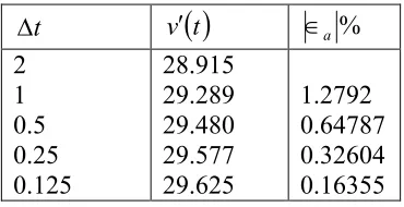
Table 2 First derivative approximations and relative errors for different ∆t values of backward difference scheme.

t

∆ v′

( )

t ∈_a%

2 1 0.5 0.25 0.125

28.915 29.289 29.480 29.577 29.625

1.2792 0.64787 0.32604 0.16355

From the above table, one can see that the absolute relative approximate error decreases as the step size is reduced. At ∆t =0.125, the absolute relative approximate error is 0.16355%, meaning that at least 2 significant digits are correct in the answer.

Finite Difference Approximation of Higher Derivatives

One can also use the Taylor series to approximate a higher order derivative. For example, to approximate f ′′

( )

x , the Taylor series is

( )

₊ =

( )

+ ′

( )(

)

+ ′′

( )( )

2 + ′′′

( )( )

3 +

2 2Δ

! 3 Δ

2 ! 2 Δ

2 x f x x f x x

x f x f x

f i i

i i

i (3)

where

x x

x_i+2 = _i+2Δ

( )

( )

( )( )

( )( )

2

( )( )

3

1

! 3 !

2 x

x f x x f x x f x f x

f i i

i i

i ∆

′′′ + ∆ ′′ + ∆ ′ + =

+ (4)

where

x x x_i−1 = _i −Δ

Subtracting 2 times Equation (4) from Equation (3) gives

( )

( )

( )

( )( )

2

( )( )

3

1

2 2f x f x f x Δx f x Δx

x

( )

( )

( ) ( )

The velocity of a rocket is given by

( )

9.8 ,0 30

Solution

The exact value of j

( )

16 can be calculated by differentiating

Knowing that

( )

Similarly it can be shown that

( )

[ ]

a

( )

t

The absolute relative true error is

100

( ) ( )

( )

( )( )

( )( )

( )( )

...

Adding Equations (6) and (7), gives

( ) ( )

( )

( )( )

( )( )

...

The velocity of a rocket is given by

( )

9.8 ,0 30

(a) Use the central difference approximation of the second derivative of ν

( )

t to calculate the jerk at t=16s. Use a step size of ∆t=2s.

Solution

The second derivative of velocity with respect to time is called jerk. The second order approximation of jerk then is

( )

_{( )}

9.8

( )

18 18

2100 10

14

10 14 ln

2000 18

4 4

−    

 

− ×

× =

ν

=453.02m/s

( )

_{( )}

9.8

( )

16

16 2100 10

14

10 14 ln

2000 16

4 4

−    

 

− ×

× =

ν

=392.07m/s

( )

_{( )}

9.8

( )

14

14 2100 10

14

10 14 ln

2000 14

4 4

−    

 

− ×

× =

ν

=334.24m/s

( ) ( )

( ) ( )

( )

2

2

14 16

2 18

16 ≈ν − ν +ν j

(

)

4

24 . 334 07 . 392 2 02 .

453 − +

=

=_0.77969m/s3

The absolute relative true error is

100 77908

. 0

77969 . 0 77908 . 0

× −

= ∈_t

=0.077992%

DIFFERENTIATION

Topic Differentiation of Continuous functions

Summary These are textbook notes of differentiation of continuous functions Major General Engineering

Authors Autar Kaw, Luke Snyder Date February 2, 2012