Journal of Post Keynesian Economics / Summer 2012, Vol. 34, No. 4 777 © 2012 M.E. Sharpe, Inc. 0160–3477 / 2012 $9.50 + 0.00.
Keynesian and Schumpeterian efficiency
in a BOP-constrained growth model
Abstract: The paper aims to contribute to the debate on specialization and growth in two forms. First, it develops a north–south model in which the ratio between the income elasticity of exports and imports in the south (which gives the rate of growth compatible with external equilibrium) depends on the Keynesian and Schumpeterian efficiencies of the pattern of specialization, as defined by Dosi et al. (1990). Second, the model is tested including the technology gap and proxies for the pattern of specialization (Keynesian and Schumpeterian efficiency) in Keynesian growth regressions. Several estimation procedures are used to test the model, among which finite mixture estimation, which allows for more robust estimations of the parameters for homogeneous groups of countries.
Key words: balance-of-payments-constrained growth, Keynesian efficiency, Schumpeterian efficiency, Thirlwall’s law.
The role of specialization in economic growth has been the subject of an enduring debate among economists of diverse schools of thoughts. The idea that the quality of exports matters is a central tenet in both the Latin American structuralist tradition1 and in the Keynesian–Shumpeterian (KS) approach to economic growth. These schools suggest that inter-national competitiveness and exports play a key role in sustaining the expansion of the economy with external equilibrium (a point stressed by Kaldor, 1978, ch. 4). Inversely, in the neoclassical tradition the specific pattern of specialization is not relevant since it assumes that trade would suffice to evenly spread productivity gains around the world.2 This view has changed in recent years and some authors of neoclassical persuasion
Gabriel Porcile is <<WHAT IS YOUR POSITION? E.G., PROFESSOR>> in <<AFFILIATION>>. Eva Yamila da Silva Catela is <<WHAT IS YOUR POSI-TION?>> in <<AFFILIATION>>.
1 Structuralist views can be found in Prebisch (1963). See also Cimoli and Porcile
(2009), Economic Commission for Latin America and the Caribbean (2007), Ocampo et al. (2009), and Rodríguez (1980).
have begun to accept as well that the quality of exports could contribute to explain why growth rates differ.3
This paper aims at contributing to the KS literature in two ways. The first one (see the next section) is by presenting a north–south model that formalizes the interrelations between the technology gap, specializa-tion, and growth. We will focus on the relationship that exists between specialization and the income elasticity of the demand for exports and imports—the elasticity ratio. We believe that such an approach highlights the key interrelations that exist between Schumpeterian and Keynesian variables in economic growth. Following the work of McCombie and Thirlwall (1994) and Thirlwall (1979), we argue that the relative rate of growth of a certain country (as compared to the rate of growth of the world economy) should equal the income elasticity ratio. In addition, follow-ing the work of Ciarli et al. (2010), Cimoli et al. (2010), and Dosi et al. (1990), among others, we will argue that the elasticity ratio is a function of the “Schumpeterian efficiency” (S) and “Keynesian efficiency” (K) of the pattern of specialization. The model allows K and S to interact though time with the technology gap so as to endogenously produce different trajectories of growth and catching up in the international economy.
The second contribution (the third and fourth sections) is to present an empirical test of the suggested model for the period 1985–2007, based on a large sample of countries and using different econometric techniques. More specifically, we focus on panel data with fixed effects and finite mixture models. The finite mixture model—which has not yet been used to test growth models—is particularly interesting since allows for identifying differences between the parameters of different groups of countries. Such groups are endogenously constructed, on the basis of the statistical analysis of their heterogeneity, not through the imposition of exogenous criteria. In all cases, we test the idea that specialization af-fects growth by including in the regressions K and S (in the third section), and the technology gap (the fourth section), along with the variables that are traditionally considered in balance-of-payments (BOP)-constrained growth models,4 namely, the terms of trade and the rate of growth of world income.
3 See Acemoglu (2009, ch. 20) and Hasuman et al. (2007)<<HASUMAN ET AL.
NOT IN REFERENCE LIST (ALSO, VERIFY SPELLING, HAUSMAN?)>>.
4 There is already a large literature on the empirics of BOP-constrained growth
The model: a Keynesian–Schumpeterian view on convergence and structural change
Keynesian and Schumpeterian efficiency and the elasticity ratio
Our point of departure is the canonical BOP-constrained growth model. One country (a small open economy) will be called “south” and the rest of the world will be called “north.” The key result of the model is that under certain assumptions, the long-run rate of growth is given by the ratio between the income elasticity of the demand for exports and imports, which is known as “Thirlwall’s law.”5 Formally,
y* p p n z
*
.
=
(
1+ +η µ)
(
− −)
+επ (1)
where y* is the southern long-run rate of growth compatible with BOP equilibrium; p is domestic inflation; p* is international inflation; n is the rate of growth of the nominal exchange rate (defined as units of lo-cal currency per international unit); z is the rate of growth of the world economy (north); η and µare negative price elasticities of north and south exports, respectively; and ε and π are positive income elasticities of southern exports and imports, respectively. There are no capital flows in the model, which implies that the long-run rate of growth cannot be based on external debt.6
Assuming that the real exchange rate remains constant, Equation (1) becomes
y* = εz= z.
π ξ (2)
Equation (2) relates the BOP-constrained rate of growth to the income elasticity ratio, defined as ξ = ε/π (recall that ε and π are income elastici-ties of exports and imports<<DELETE PARENTHETICAL? THIS WAS SAID JUST ABOVE>>). From this result, it is possible to obtain the southern relative rate of economic growth in equilibrium:
5 Thirlwall’s law is an important result of Keynesian growth models in open
econo-mies, which has been extensively discussed in the literature. A detailed discussion of the basic model can be found in McCombie and Thirlwall (1994, ch. 3). See also Dutt (2002) and Setterfield and Cornwall (2002).
6 Periods in which the external debt rises should be followed by periods in which
y z
*
.
= ξ (3)
Equation (3) represents the simplest BOP-constrained growth model relating relative growth to the income elasticity ratio. This is the demand-led rate of growth: to keep the trade balance in equilibrium, relative growth in the south cannot exceed the level defined by the ratio between the income elasticity of exports and imports.
A crucial aspect to be addressed from a theoretical point of view is what forces affect the evolution of the income elasticities of the demand for exports and imports. We will argue that these elasticities depend on what Dosi et al. (1990) has called the Keynesian and Schumpeterian efficiencies of the specialization pattern. The concept of Keynesian ef-ficiency (K) captures the direct demand-side effects of export growth and is represented by the share in the country’s total exports of sectors whose international demand grows at higher rates than the world aver-age (dynamic sectors in terms of demand growth). A country may have a high K because of its past achievements in technological competitive-ness, active pro-export policies, preferential trade agreements, and/or just because it had good luck in the commodity lottery.
The concept of Schumpeterian efficiency (S), in turn, captures the ability of each country to adjust to changes in demand patterns and technology. This ability is a function of the country’s technological capabilities, which provide the basis for creating new markets and sustaining international competitiveness as new goods, new processes, and new actors continu-ously challenge the prevailing distribution of market shares.7 To remain competitive in the domestic and international markets (and to sequentially move toward sectors in which demand grows faster) the country must be able to innovate, learn, and adopt new technology at least at the same pace as its competitors.8 We use in this paper as a proxy of Schumpeterian efficiency the share of high-tech exports in the country’s total exports (dynamic sectors from a technological point of view).9
In addition, Schumpeterian efficiency allows the country to more easily overcome supply-side constraints as the economy grows. In a
conven-7 A point stressed by Schumpeter (1952, ch. 9)<<NOT IN REFERENCE LIST>>
in his classical work.
8 If competitiveness is solely based on natural resources or cheap labor, sooner or
later the country will lose ground in the international markets, as suggested by the economic history of Latin America (Bértola and Porcile, 2006; Ocampo et al., 2009).
9 We adopted the definition of high-tech exports suggested by Hatzichronoglou
tional model the supply constraint is the general case, as it is assumed the validity of Say’s law. The demand-side always adjusts to the natural rate of growth of labor supply and labor productivity (for a discussion, see Setterfield, 2009<<NOT IN REFERENCE LIST>>). We take the opposite view, in which the influence of supply depends on its effects on effective demand. This excludes the automatic adjustment mechanisms between supply and demand implicit in Say’s law. In the context of our model, productivity growth and structural change only affect economic growth if they change the income elasticity ratio, thereby allowing for a higher share of the south in domestic and foreign effective demand.10
The relationship between export growth, K and S can be expressed in a formal way as follows:
y* =µ
(
p−p* −n)
+αK+βS+ψz. (4)For simplicity, we have adopted a separable, linear form for the growth equation, although other specifications are possible. In Equation (4) µ = 1 + η + µ (whose sign is negative if Marshall–Lerner holds), K is the share in total exports of sectors which are dynamic from a demand-side point of view, and S is the share in total exports of sectors which are dynamic from a technological point of view. The positive parameters α and β give the effect of K and S, respectively, on the income elasticity of exports and imports. We expect both parameters to be positive, as a higher K and S raise the income elasticity of exports and curb the income elas-ticity of imports, favoring economic growth in equilibrium in the south. Finally, the positive parameter ψ captures other influences related to the growth of international demand not related to the two types of efficiency defined above.11 The variables K and S are in natural logarithms. If the real exchange rate is stable (i.e., p – p* – n = 0), we get
y* = αK + βS + ψz. (5)
10 For instance, in the canonical neoclassical growth model, when population
grows faster, wages will fall respecting<<WITH REGARD TO? REGARDING?>> the rental price of capital and full employment will be attained with a higher rate of growth of investment. In the KS model set forth in this paper (and in Keynesian mod-els in general), on the other hand, faster population growth may reduce wages, but there is no automatic mechanism that transforms this fall into a proportional rise in capital accumulation. In the BOP-constrained growth model, if income elasticities do not vary with wages, then the latter will not affect the rate of growth of exports or the rate of economic growth in equilibrium.
11 Note that the coefficient of z in the econometric model is ψ and not ξ because we
In sum, economic growth depends on the forces that shape the external constraint, related to the growth of international demand, along with the technological capabilities necessary to transform the specialization pattern, avoid falling behind the international technological frontier, and remain competitive in fast-growing markets.
The dynamics of specialization and growth
The dynamics of Schumpeterian efficiency
We now focus on the dynamics of K and S, drawing from the Schum-peterian literature (for a review, see Cimoli and Porcile, 2009). This analysis is central to the discussion of convergence and divergence, and for understanding the formation of relatively homogeneous groups of countries in the international economy.
We model the participation of high-technology sectors in the export structure as a function of leads and lags in international innovation and diffusion of technology.12 We express these leads and lags in terms of the technology gap, G = ln(TN /TS), the ratio between technological capabili-ties in the south (TS) and in the north (TN). A proxy for the technology gap is provided by the ratio between investments in research and development (R&D) as a percentage of gross domestic product (GDP) in the country on the technological frontier and the same percentage in the laggard economy. Although there is no single measure of the technology gap that could be considered satisfactory, R&D is widely used in the literature as a proxy for and a crucial component of these capabilities (see Dosi et al., 1990; Katz, 1987, 1997; Lall, 2000; UNCTAD [United Nations Conference on Trade and Development], 2003, 2006). Formally,
S = r – tG. (6)
Since this is a north–south model in which the north is the technological leader, it will be true that 1 < G. In Equation (6), t captures the influence of the technology gap on the share of high-tech exports in total exports. Clearly, if the technology gap is completely eliminated, then G = 1 and S = r−t. Therefore, r−t > 0 represents the international distribution of high-tech exports in the absence of technological asymmetries. Dif-ferentiating Equation (6) with respect to time renders
S¾ = –tG¾. (7)
12 Several works have linked the technology gap to competitiveness and growth—
In other words, changes in the technology gap drive S. It is therefore necessary to look in more detail at the evolution of G. Fagerberg (1994), Narula (2004), and Verspagen (1993) suggest that the initial level of the gap is important for the evolution of G, but it is not clear whether it has a positive or a negative effect. On the one hand, a high-technology gap is an opportunity for adopting the existing technology and in this sense it boosts the potential rate of technical change in the South. Therefore, the higher the north–south gap, the higher will be technological spill-overs from the north to the south. On the other hand, if the technology gap is too high, the south would not have the minimum capabilities required to effectively benefit from technological spillovers.13 In this case the gap has a negative effect on southern catching up. In subsection (b.3)<<CLARIFY SUBSECTION MEANT (SECTION NUMBERS ARE NOT USED PER JOURNAL STYLE) / IN THE EQUILIBRIA AND STABILITY SECTION?>> we discuss the implications of these different assumptions about the influence of the gap for the stability of the system. In both cases, it should be observed that there is nothing automatic in catching up or falling behind, as changes in the technology gap depend on the developing country’s own efforts to absorb foreign technology.
A second variable affecting the evolution of the technology gap is the Keynesian efficiency of the specialization pattern. Following the Kaldorian tradition, we assume that there exists increasing returns to economic growth, and in particular from export growth. Higher Keynesian efficiency favors the process of catching up by heightening investment (with its related components of embodied and disembodied technology) and the various forms of learning that accompanies economic growth, such as learning by doing, learning by using, and learning by exporting. Formally,
G¾ = g – lG – nK. (8)
The parameters g(the autonomous component in the evolution of the technology gap) and n (which captures the effects of growth in the south in reducing the technology gap) are both positive. As discussed before, the sign of the parameter l (which captures the net effect of technological spillovers from north to south) is ambiguous.14 In a very concise form, their values depend on the characteristics of the National
13 See UNCTAD (2006) for a detailed discussion of this point.
14 l expresses the capacity of the country to transform opportunities for adopting
System of Innovation (NSI), that is, the general framework that shapes in each country the stimulus to invest in technology, R&D, and educa-tion.15 Countries differ widely in terms of their NSI, and this leads to large differences in their efforts for catching up with the international technological frontier.
Using Equation (8) and in (7) renders
S= − +t g l
(
G+nK)
. (9) And using Equation (6) in (9):<<RENDERS? GIVES? GIVES US?>>
S= − +
(
−S)
+ K
t g l
t r n . (10)
The dynamics of Keynesian efficiency
We have mentioned that the rate of change of S depends on K. At the same time, there is a feedback effect, from S to the rate of change of K. We will assume that this effect is not linear. After a critical value of the share of high-tech sectors in total exports, the ability of the country to increase its market share in fast-growing markets increases at a decreas-ing rate. Formally,
K=S
(
φ−S)
. (11)The parameter φ captures the influence of technological capabilities on the ability to compete and get a higher share of the international effective demand through time.
Equilibria and stability
Equations (10) and (11) form a system of differential equations that endogenously produce two equilibrium positions defined by
S1* =0, K1* = g t lr−
nt (12)
S2* =φ, K2* = g t l φ r+
(
−)
.nt (13)
The Jacobian <<WORD MISSING? JACOBIAN WHAT? MA-TRIX?>> of the dynamic system in equilibrium is as follows:
J= − −
φ l2S* nt0. (14)
It is straightforward that the trace is negative (–l, if we assume l > 0), while the sign of the determinant [–(φ – 2S*)nt] depends on the value of S*. The first equilibrium value of Schumpeterian efficiency (S
1* = 0), given by Equation (12), produces a negative determinant and therefore a saddle point (unstable except for the too specific set of initial values that defines the stable branch). On the other hand, the second equilibrium value (at S2* = φ), given by Equation (13), renders a positive determinant (φnt), and hence a locally stable system. In addition, if the nonlinearity does not exist and the rate of growth of K always increases with S, then the equilibrium will be a saddle path and hence unstable. Although this specific case is not discussed in this paper, such a situation may represent the case of several least developed economies whose participation in fast-growing international markets decreases continuously through time.
A similar story emerges when the country lacks the minimum tech-nological capabilities required for catching up and hence l is negative. In this case, the higher the technology gap, the higher will be the rate at which the country falls behind the international technological frontier (Equation (8)). The Jacobian <<MATRIX?>> (14) shows that the trace is positive and therefore the system is unstable. Not only the rates of growth would differ across countries, but such differences would increase through time, heightening the asymmetries between north and south in the international economy.
In sum, the suggested KS model argues that the technology gap and the pattern of specialization are endogenously determined and drive ex-port growth, which in turn defines the rate of economic growth through Thirlwall’s law. In the next section, we test empirically this hypothesis based on different estimation procedure, working with a database com-prising a large sample of countries for the period 1985–2007.
Growth and specialization: empirical analysis
The previous discussion has stressed the interactions between growth, technology, and the pattern of specialization. From the model emerges a set of relations that will be tested in this section. The hypotheses to be tested are the following:
2. Since the influence of K and S on growth is related to the influ-ence of specialization on the income elasticity of the demand for exports and imports, then the rate of growth of exports should as well be a function of K, S, the terms of trade, and the rate of growth of the international economy;
3. Since growth depends positively on K and S, and the latter variables<<WHICH LATTER VARIABLES? K AND S ONLY ONES MENTIONED / “...DEPEND POSITIVELY ON K AND
S, WHICH IN TURN DEPEND...”?>> in turn depend negatively on the technology gap, we expect to find a negative relation be-tween economic growth and the technology gap. The same can be said as regards the rate of growth of exports. In other words, the hypotheses defined in 1 and 2 above should be confirmed when we replace K and S by the technology gap on the right-hand side of the growth equations.
Growth and specialization: fixed effect model
In this item<<WHAT ITEM? IN THIS SUBSECTION? IN THE FIXED EFFECT MODEL?>> we address empirically the relationship between specialization and growth, testing Equation (4). First, we use conventional panel data estimation procedures (fixed effects). Second, we use the finite mixture methodology, which allows for endogenously identifying groups of countries and estimating different parameters for these groups.16
The estimated equation is a follows:
yi =β0 +α
( )
Ki +β( )
Si +ψ( )
z +µ( )
tot i+ei,(15)
where ei is a white noise error term and the indicators of the pattern of specialization, K and S, are taken in natural logarithms. This equation opens the black box of the elasticity ratio to make it a function of K and S. The variables y and z are the real rates of GDP growth of country i and the world economy, respectively; Si is the share of high-tech sectors in total exports (Schumpeterian efficiency) and Ki is the share of sectors whose demand grew at higher rates than the average demand growth in the world economy (Keynesian efficiency; see Appendix A). The
valid-16 The raw data obtained from the TradeCan2009, WTO<<DEFINE / WORLD
ity of Marshall–Lerner is an empirical matter that requires to be tested by including the variation of the terms of trade (tot) in the estimated equation.17 The terms of trade index is defined as the ratio of the average prices on goods and services exported to the average prices on goods and services imported, px/pm, where px is the export price index and pm is the import price index.18 In addition, the rate of growth of the world economy is included with a view to capturing (through the parameter ψ) other factors that could affect the elasticity ratio but which are not related to the Schumpeterian and Keynesian efficiencies.
Two estimation procedures were applied: fixed effects and random ef-fects. However, since the Hausman test proved that the fixed effect model is the correct one, we only report the results of this model in Table 1.19
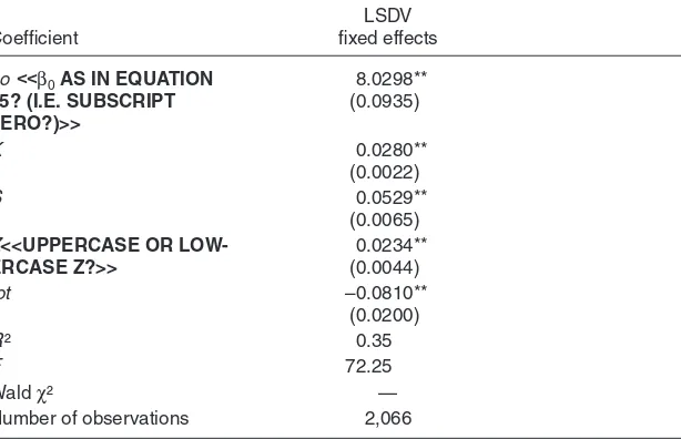
The results <<SHOWN IN TABLE 1?>> are compatible with the hy-pothesis that the pattern of specialization affects growth through its two dimensions (Schumpeterian and Keynesian). The variable coefficients are all positive, as expected, and significant at the 1 percent level. In ad-dition, it can be seen that the technological dimension of international competitiveness has a stronger leverage on growth than pure demand shocks. Last but not least, the variable terms of trade is significant and has the expected sign (which is negative, suggesting that the Marshall– Lerner condition is valid).
To the extent that the pattern of specialization affects growth through the BOP constraint, we tested the effect of K and S in the growth rate of exports by means of the following linear equation:
xi=βx0+α
( )
Kxi +β( )
Sxi +ψx( )
z +µx( )
tot i+ei. (16)The suffix x indicates that the parameters are those of the export growth equation. The results of the estimation can be seen in Table 2. The coef-ficients of K and S are significant and have the expected sign, with higher values than in the growth equation.
In sum, the econometric results are compatible with the predictions of the BOP-constrained growth model, in which the pattern of specializa-tion matters for growth. The evidence suggests that the Keynesian and
17 This is the reason we estimated Equation (5) rather than Equation (6).
18 The data are from the World Development Indicators<<ANY YEAR IN
PAR-TICULAR? REFERENCE NEEDED?>> provided by the World Bank.
19 The χ² statistics (57, 79) of the Hausman test allows for rejecting the idea
Schumpeterian dimensions were both relevant for export and GDP growth between 1985 and 2007.
Growth and specialization: finite mixture model
Along with panel data techniques, we tested the model using a finite mixture procedure. This procedure has not yet been used in the literature to test growth models. However, it has some very interesting properties as allows for controlling the heterogeneity of the data. In effect, if the data are generated from a density function with finite mixtures, in which different groups show different parameters, then estimations based on the hypothesis of a simple probability density function produce biased estimates (Frühwirth-Schnatter, 2006). For this reason it is preferable to model the statistical distribution assuming that there exists a mixture or combination of distributions. A finite mixture may be a way of modeling Table 1
GDP growth: estimation results, 1985–2007
Dependent variable: GDP growth, y
Coefficient
LSDV fixed effects
βo <<β0AS IN EQUATION 15? (I.E. SUBSCRIPT ZERO?)>>
8.0298** (0.0935)
K 0.0280**
(0.0022)
S 0.0529**
(0.0065)
Z<<UPPERCASE OR LOW-ERCASE Z?>>
0.0234** (0.0044)
tot –0.0810**
(0.0200)
R ² 0.35
F 72.25
Waldχ² —
Number of observations 2,066
Source: Author’s estimations based on TradeCAN<<FOOTNOTE 16 SAYS
Trade-CAN2009>> and Penn World Table-mark 6<<WHAT IS “mark 6” (FOOTNOTE 16
SAYS “Table 6.3”)>> databases.
Notes:<<WHAT DOES LSDV IN 2ND COLUMN HEADING STAND FOR?>>βo
<<OR IS IT β0?>> = <<WHAT DOES β and o STAND FOR?>>K = share of sectors
the data in a more flexible form, with each mixture component providing a local approximation to some part of the true distribution.
The regression model with finite mixtures can be written as
yij = αj + β1j Kijt + β2j sijt + β3j Zijt + β4j totijt + β5j yt–1ijt + uijt, (17) i = 1, 2, ..., n; j = 1, 2, ..., J; t = 1985, ..., 2007,
where αj is the intercept for component j, yijt is the endogenous variable for country i in component j in year t (GDP per capita growth rate), Sijt<<THIS IS LOWERCASE s IN EQUATION 17>> is the share of high-tech sectors in total exports for country i in component j in year t; Kijt is the share of sectors whose demand grew at higher rates than the average demand growth in the world economy for country i in compo-nent j in year t; totijt is the terms of trade for country i in component j in year t; zjt<<Z IS UPPERCASE IN EQUATION 17 / VERIFY USE
THROUGHOUT>>is the rate of growth of the world economy for Table 2
The rate of growth of exports and specialization
Dependent variable: export growth
Coefficient
LSDV fixed effects
βxo<<βx0 (i.e., x0 AS IN
EQUATION 16?>>
16.45** (0.0146)
Kx 0.1134**
(0.0050)
Sx 0.0725**
(0.0146)
zx<<UPPERCASE OR
LOW-ERCASE Z?>>
0.0756** (0.0098)
tot 0.0019**
(0.0004)
R ² 0.40
F 324.96**
Number of observations 1,927
Source: Author’s estimations based on TradeCAN and Penn World Table-mark 6 databases.
Notes:<<WHAT DOES LSDV IN 2ND COLUMN HEADING STAND
FOR?>><<WHAT DOES β STAND FOR? WHAT DOES x and o STAND FOR?>>
component j in year t; and yt–1ijt is the lagged dependent variable. We in-clude the lagged dependent variable because it absorbs the time-invariant properties, capturing the fixed effects. Finally, uij is the error term, whose variance sij2 is assumed to be normal and homoskedastic within compo-nents, but probably heteroskedastic between components.20
As mentioned, we used the finite mixture model (FMM) to estimate the parameters for the variables of our growth model (K and S) without having to arbitrarily separate countries in different groups. The FMMs are estimated using maximum likelihood, while cluster-corrected robust standard errors are used throughout for inference purposes. These are implemented by the Stata package fmm (Deb, 2008).
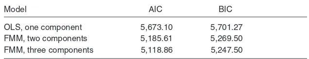
The estimation procedure requires, first, identifying the number of groups that best suits the heterogeneity of the data. The dependent vari-able for group formation is the GDP per capita. Tvari-able 3 presents two statistics that measure the quality of adjustment, computed with a view to deciding whether the estimation should be done with just one component (which corresponds to ordinary least squares), <<OR?>> two or three components (to be estimated by means of the FMM). The statistics used to choose the appropriate model are the Akaike information criterion (AIC) and the Bayesian information criterion (BIC).21
It should be recalled that the lower the AIC and BIC indexes, the better is the adjustment of the model. Both statistics clearly point out that the best model is the FMM with three components.
Another form of testing the number of groups that should be included in the estimation procedure is through the LM<<DEFINE>> statistic. If the fy function takes the form of a density mixture for all y∈y, then
20 The methodology allows for assuming different probability distributions for the
error term. In our model, we assumed a normal distribution.
21 See Akaike (1973) and Schwarz (1978).
Table 3
Number of components in the model: AIC and BIC
Model AIC BIC
OLS, one component 5,673.10 5,701.27 FMM, two components 5,185.61 5,269.50 FMM, three components 5,118.86 5,247.50
fy=η1 1f y
( )
+ + ηjfj( )
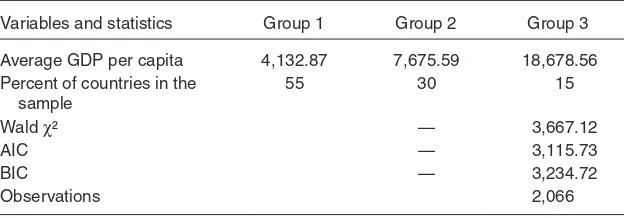
y (18) In this equation, fj (y) is a density probability function for all j = 1, ..., J. The density fj (y) is called “component density,” where J is the number of components. The parameters η1, ..., ηj are weights, whose distributions are given by the vector η = (η1, ..., ηj). The null hypothesis is that the fY <<y IS LOWERCASE IN EQUATION 18>> has two components as against<<CLARIFY “AS AGAINST” / AS COMPARED TO? VER-SUS?>> the alternative of having three components. A χ² test provides a significant statistic (χ² = 116,87), allowing us to conclude in favor of the model with three components.Table 5 shows the results of group formation based on the FMM. Group 1, which has the lowest income per capita, represents about 45 percent of the countries of the sample, while Group 3, with the high-est income per capita, represents about 13 percent. The middle-income Group 2, which includes all the Latin American countries, responds for about 41 percent of the countries. These groups are endogenously formed by the statistical analysis of the sample variance.22
A few points are worthwhile stressing. First, all the Latin American countries are in Group 2 and none of them migrated to a different group. Chile managed to move from the middle to the top position within Group 2, while Bolivia and Nicaragua moved toward the lower end—with Bolivia in a transitional position between Groups 2 and 1. But all of them remained in the same group<<DELETE? REPEAT OF WHAT SAID IN 2ND SENTENCE OF PARAGRAPH?>>. Inversely, there is strong intergroup mobility in the case of Asia and some European economies.
22 The countries included in each group are available on request of the authors.
Table 4<<NOT CITED / INDICATE WHERE TO MENTION TABLE 4 IN THE TEXT>>
Groups in the sample: results from the finite mixture model
Variables and statistics Group 1 Group 2 Group 3
Average GDP per capita 4,132.87 7,675.59 18,678.56 Percent of countries in the
sample
55 30 15
Wald χ² — 3,667.12
AIC — 3,115.73
BIC — 3,234.72
Observations 2,066
In effect, Indonesia and China moved from Group 1 to Group 2 in 1992 and 1998–99, respectively. Korea, in turn, migrated from Group 2 to Group 3. In Europe, Ireland and Spain moved from Group 2 to Group 3 in 1995–96, and so did Greece and Portugal by the end of the period. Last but not least, poor countries in Group 1 were unable to improve their position and escape toward a higher group. Most African countries and a significant number of Asian countries are in this highly unfavorable condition, which seems to represent a kind of underdevelopment trap. In terms of the model presented in the previous section, these results suggest that some countries succeed<<SUCCEEDED?>> in changing the value of the parameter φ that defines the equilibrium levels of S and K.
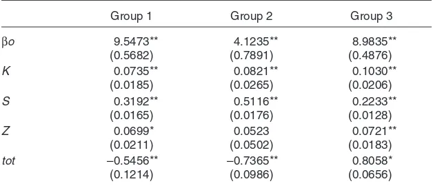
After forming the groups, the next step is to run an FMM regression for the growth model, whose results are presented in Table 5. Some of the conclusions that can be drawn from Table 5 are the following:
1. The coefficients obtained using the FMM are much higher than those obtained with the fixed effect model. All the groups show pos-itive and significant coefficients for the variables S and K. Schum-peterian efficiency in all cases has a larger<<GREATER?>>
impact on growth than the Keynesian one<<KEYNESIAN EFFICIENCY?>>.
2. The coefficient of Schumpeterian efficiency for Groups 1 and 2 are higher than for Group 3. Efforts for export diversification Table 5
GDP growth: finite mixture regression results, 1985–2007
Group 1 Group 2 Group 3
βo 9.5473**
Source: Author’s estimations based on TradeCAN and Penn World Table-mark 6 databases.
toward more technologically intensive sectors can be expected to have a larger<<GREATER?>> impact on growth in developing economies.
3. The terms of trade show the expected negative signal associated with the Marshall–Lerner condition, except for the high-income economies (Group 3), where the coefficient does not significantly differ from zero. This may be explained by the fact that the ad-vanced economies compete in high-tech sectors where innovation is more important than price competitiveness.
The FMM methodology confirms the results arising from our previous estimations respecting<<REGARDING?>> the significance and signal of the variables of the model. Still, the FMM procedure has a critical advantage, namely, it allows for obtaining specific coefficients for each group, capturing in a more precise form the influence of the countries’ productive structures on growth. Differences in the coefficients across groups can be interpreted in terms of the different levels of technological and productive development that each region has achieved.
It is worthwhile stressing that estimating the parameters for endogenous groups of countries cannot be equated with the formation of convergence clubs, as suggested in neoclassical convergence theory (Quah, 1996). Our model is based on a KS perspective in which each country has its own long-run rate of growth and there is no reason for the poor countries to catch up with the rich countries. We expect in equilibrium different patterns of specialization and persistent technological asymmetries. The model does not consider the possibility of decreasing returns to capital accumulation. Convergence is possible on the basis of international technological diffusion and spillovers, along with industrial policies that strengthen the NSI and international competitiveness.
Growth, exports, and the technology gap
The model presented in the second section points out that changes in the technology gap are the ultimate determinants of changes in K and S. This suggests the possibility of running a regression in which both economic growth and export growth will be a function of the technology gap, along with the terms of trade and growth in the global economy. In other words, the technology gap may replace K and S in the structural Equations (4) and (16).
To test for the role of the technology gap in economic growth, we need an adequate proxy for this variable—such as K and S are proxies for the dynamism of the pattern of specialization. Some authors have used the GDP per capita ratio between two countries (the technological leader and the laggard) as a measure of the technology gap (Fagerber<<SPELLED FAGERBERG IN REFERENCE LIST>>, 1988<<1994 IN REFER-ENCE LIST>>). In Appendix B, we present the results of a panel data regression of K and S on this indicator of the technology gap, using the U.S. GDP per capita as a benchmark. The results confirm the existence of a positive, significant relation between specialization and technology. However, the GDP per capita ratio as a proxy of the technology gap may produce problems of endogeneity in growth equations. Moreover, the technology gap is just part of the determinants of GDP per capita; it would be preferable to have a direct, learning-based indicator of the technology gap (UNCTAD, 2006). With this objective, we created a new proxy, which is the ratio between investment in R&D (R&D as a percentage of GDP) in the leader country (the United States) and the same kind of investment in the laggard country.23 This proxy was then included as an independent variable in the fixed effect models of the previous section.
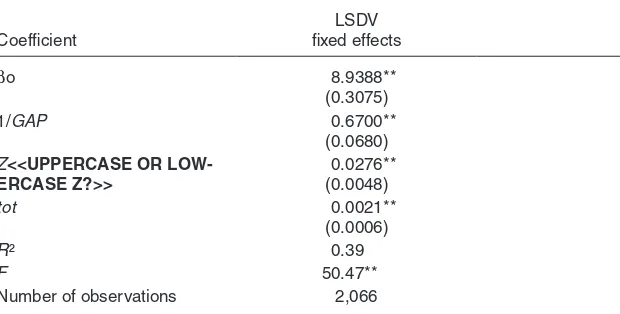
Table 6 clearly shows that the lower the technology gap, the higher the rate of economic growth. It should also be observed that the coefficient of the technology gap is much higher than those found for K and S in the regressions presented above. The terms of trade, on the other hand, do not conform to Marshall–Lerner in this case.
23 The use of R&D investment as a proxy for technological capabilities has many
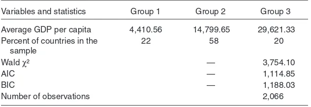
We also run a similar regression with the three groups identified by the FMM, which divided the sample of countries according to their GDP per capita. Some interesting results emerge from the FMM, presented in Tables 7 and 8. Table 7 presents the outcome of the regressions, and Table 8 presents the data about the homogeneous groups formed using FMM.
What can be learned from these results? First, for all groups of coun-tries the technology gap is a significant determinant of economic growth. Second, there exists a nonlinearity in the relationship between the gap and economic growth. In the groups with lower GDP per capita (Groups 1 and 2), the higher the gap, the lower is the rate of growth. On the other hand, in Group 3 (the group with the highest GDP per capita), the gap is negatively related to growth: ceteris paribus, laggard countries grow at higher rates than the leaders. This result tends to confirm the point raised by Narula (2002<<2004 IN REFERENCE LIST>>) and Verspagen (1993) about nonlinearities in the international diffusion of technology. For the group of developed economies, where in general the gap is low, there will be convergence (laggards mostly benefit from technological Table 6
Growth and the technology gap: fixed effects model
Dependent variable: GDP growth
Coefficient
LSDV fixed effects
βo 8.9388**
(0.3075)
1/GAP 0.6700**
(0.0680)
Z<<UPPERCASE OR LOW-ERCASE Z?>>
0.0276** (0.0048)
tot 0.0021**
(0.0006)
R ² 0.39
F 50.47**
Number of observations 2,066
Source: Author’s estimations based on TradeCAN and Penn World Table-mark 6 databases.
Notes: <<WHAT DOES LSDV IN 2ND COLUMN HEADING STAND FOR?>>βo
<<OR IS IT β0?>> = <<WHAT DOES β and o STAND FOR?>> ; 1/GAP =
<<DE-FINE>>; z<<LOWERCASE OR UPPERCASE Z?>> = growth rate of the world
Table 7
Growth and the technology gap: finite mixture procedure
Group 1 Group 2 Group 3
βo | 7.5504**
<<WHAT DOES THE | (VERTICAL LINE) INDICATE BEFORE THE FIRST NUMBERS IN GROUP 1? IS IT AN ERROR AND NEEDS TO BE
DELETED?>>Notes:<<WHAT DOES β and o STAND FOR?>>; 1/GAP =
<<DE-FINE>>; z<<LOWERCASE OR UPPERCASE Z?>> = growth rate of the world
economy; tot = terms of trade. Standard deviations are shown in parentheses. ** and * sig-nificant at the 1 percent and 5 percent levels, respectively.
Table 8
Groups in the sample: results from the finite mixture model
Variables and statistics Group 1 Group 2 Group 3
Average GDP per capita 4,410.56 14,799.65 29,621.33 Percent of countries in the
sample
Note: AIC = Akaike’s infomation criterion; BIC = Bayesian information criterion.
spillovers from the leading economies). Inversely, when the gap is high, as in Groups 1 and 2, differences in international competitiveness related to the gap prevail over technological diffusion, leading to divergence rather than convergence.
Finally, we tested for a positive association between export growth and the technology gap. The results, presented in Table 9, confirm the existence of such a relationship. Again, this result is not incompatible with the predictions of the KS model of the second section.
different forms, including direct regressions of K and S on the technol-ogy gap, and regressions of economic growth and export growth on the technology gap, using both the FEM<<SPELL OUT (ABBREVIATION NOT USED ELSEWHERE) / FIXED EFFECTS MODEL?>> and the FMM.
Concluding remarks
This paper contributes to the Keynesian–Schumpeterian literature on economic growth in two forms. First, by developing a north–south model that makes explicit how the technology gap and the Keynesian and Schumpeterian efficiencies of the specialization pattern interact, shap-ing the income elasticity ratio—and therefore the BOP-constrained rate of growth. The model allows for analyzing the effect of demand shocks and policy interventions (particularly in the technological field) on the process of international convergence or divergence in GDP per capita and technological capabilities.
We also tested the different relations between the variables set forth in the model (and in the KS literature in general) by using a fixed effects Table 9
Export growth and the technology gap
Dependent variable: export growth
Coefficient
LSDV fixed effects
βxo 17.4082**
(0.0725)
1/GAP 1.6041**
(0.1628)
zx 0.0604**
(0.0113)
tot 0.0070**
(0.0011)
R ² 0.28
F 53.60
Number of observations 539
Source: Author’s estimations based on TradeCAN and Penn World Table-mark 6 databases.
Notes:<<WHAT DOES LSDV IN 2ND COLUMN HEADING STAND FOR?>>βxo
<<OR IS IT βx0?>> = <<WHAT DOES β, x, and o STAND FOR?>>; 1/GAP =
<<DE-FINE>>; z<<LOWERCASE CORRECT? (SOME OTHER TABLES ARE
UPPER-CASE)>> = growth rate of the world economy; tot = terms of trade. Standard deviations
model and an FMM in a sample of 107 countries<<NOT STATED IN TEXT / SHOULD INFORMATION BE INCLUDED IN DISCUS-SION OF COUNTRIES?>> for the period 1985–2007. In very concise terms, we found favorable evidence to the idea that (1) Keynesian and Schumpeterian efficiencies (using the variables K and S as proxies) foster growth, (2) these efficiencies play a role in export growth, (3) they are closely related to proxies of the technology gap, (4) growth depends on the technology gap along with the other variables of demand-led growth models (real exchange rate and global growth), and (5) export growth is encouraged too by a lower technology gap.
The use of the FMM allowed us to divide the sample of countries into homogeneous groups according to their GDP per capita. By doing so, some differences could be identified regarding the evolution of conver-gence. In particular, policies of structural change seem to be more im-portant in the case of developing economies whose lower technological capabilities render a weak Harrodian multiplier. It was also found that convergence occurs within the group of economies with higher levels of GDP per capita (Group 3), while divergence prevails in the other two groups. This provides favorable evidence to those authors who have emphasized the existence of nonlinearities and asymmetries in the re-sponse to the technology gap in the international economy, in which the process of catching up is more difficult for economies that are far from the technological frontier.
Our results suggest that the old structuralist concern with the specific form in which countries integrate to the world economy seems thoroughly justified. In particular, policies aimed at encouraging exports should be complemented by industrial and technology policies fostering structural change in favor of technology-intensive sectors.
REFERENCES
Acemoglu, D. Modern Economic Growth. Princeton: Princeton University Press, 2009.
Akaike, H. “Information Theory and an Extension of the Maximum Likelihood Principle” In B.N. Petrov and F. Csaki (eds.), Second International Symposium on Information Theory.<<VERIFY PUBLISHED TITLE / PROCEEDINGS OF...?>> <<PUBLISHER AND PUBLISHER’S LOCATION>>, 1973, <<PAGE RANGE OF CHAPTER>>.
<<NOT CITED / CITE OR DELETE>>Albuquerque, E.M. “Inadequacy of Tech-nology and Innovation Systems in the Periphery.” Cambridge Journal of Economics, 2007, 31 (5), 669–690.
Amable, B. “International Specialization and Growth.” Structural Change and Eco-nomic Dynamics, 2000, 11 (1), 413–431.
<<NOT CITED / CITE OR DELETE>>Araujo, A., and Lima, G.T. “A Structural Economic Dynamics Approach to Balance-of-Payments-Constrained Growth.” Cam-bridge Journal of Economics, 2007, 31 (5). 755–774.
Arellano, M. Panel Data Econometrics. New York: Oxford University Press, 2003. <<NOT CITED / CITE OR DELETE>>Bell, M., and Pavitt, K. “Technological Accumulation and Industrial Growth: Contrasts Between Developed and Developing Countries.” Industrial and Corporate Change, 1993, 2 (1), 157–210.
Bértola, L., and Porcile, G. “Convergence, Trade and Industrial Policy: Argentina, Brazil and Uruguay in the International Economy, 1900–1980.” Revista de Historia Económica—Journal of Iberian and Latin American Economic History, 2006, 24 <<ISSUE AND/OR SEASON>>, 120–150.
Bértola, L.; Higachi, H.; and Porcile, G. “Balance-of-Payments-Constrained Growth in Brazil: A Test of Thirlwall’s Law, 1890–1973.” Journal of Post Keynesian Econom-ics, Fall 2002, 25 (1), 123–140.
<<NOT CITED / CITE OR DELETE>>Capdevielle, M. “Globalización, Espe-cialización y Cambio Estructural en América Latina” [<<PROVIDE ENGLISH TRANSLATION / IT IS THE STYLE OF THE JOURNAL TO KEEP THE ORIGINAL AND INCLUDE THE TRANSLATION IN BRACKETS>>]. In M. Cimoli (ed.), Heterogeneidad Estructural, asimetrías Tecnológicas y Crecimiento en América Latina [<<PROVIDE ENGLISH TRANSLATION>>]. Santiago: BID-CEPAL, 2005, <<PAGE RANGE OF CHAPTER>>.
Castellacci, F. “Technology Gap and Cumulative Growth: Models and Outcomes.” International Review of Applied Economics, 2002, 16 (3), 333–346.
Ciarli, T.; Lorentz, A.; Savona, M.; and Valente, M. “Structural Transformation in Production and Consumption, Long Run Growth and Income Disparities.” WP. mimeo<<WHICH / WORKING PAPER OR MIMEO?>>, Max Planck Institute, <<CITY / COUNTRY>>, 2010.
Cimoli, M., and Porcile, G. “Sources of Learning Paths and Technological Capabili-ties: An Introductory Roadmap of Development Processes.” Economics of Innovation and New Technology, 1476–8364<<WHAT DO THESE NUMBERS INDI-CATE?>>, 2009, 18 (7), 675–694.
Cimoli, M.; Porcile, G.; and Rovira, S. “Structural Convergence and the Balance-of-Payments Constraint: Why Did Latin America Fail to Converge?” Cambridge Journal of Economics, 2010, 34 (2), 389–411.
Deb, P. “Finite Mixture Models.” Summer North American Stata User’s Group Meet-ings 2008. 2008<<PAPER PRESENTED AT...? PROVIDE LOCATION WHERE MEETINGS WERE HELD AND MONTH AND DAY(S) FOR MEETINGS>> Dosi, G.; Pavitt, K.; and Soete, L. The Economics of Technical Change and Interna-tional Trade. New York: Harvester Wheatsheaf, 1990.
Dutt, A.K. “Thirwall’s Law and Uneven Development.” Journal of Post Keynesian Economics, Spring 2002, 24 (3), 367–390.
<<NOT CITED / CITE OR DELETE>>Economic Commission for Latin America and the Caribbean. Una Década de Luces y Sombras: América Latina y el Caribe en los Años Noventa [<<PROVIDE ENGLISH TRANSLATION>>]. Bogotá: Alfao-mega, 2001.
———. Progreso Técnico y Cambio Estructural en América Latina [<<PROVIDE ENGLISH TRANSLATION>>]. Santiago: CEPAL-IDRC, 2007.
Frühwirth-Schnatter, S. Finite Mixture and Markov Switching Models. New York: Springer, 2006.
Hatzichronoglou, T. “Revision of the High-Technology Sector and Product Classifica-tion.” Technology and Industry Working Paper no. 1997/2, Organization for Economic Cooperation and Development Science, Paris, 1997.
Kaldor, N. Further Essays on Economic Theory. London: Duckworth, 1978.
Katz, J. Technology Generation in Latin American Manufacturing Industries: Theory and Case-Studies<<HYPHEN CORRECT, OR CASE STUDIES?>> Concerning Its Nature, Magnitude and Consequences. London, Macmillan, 1987.
———. “Structural Reforms, the Sources and Nature of Technical Change and the Functioning of the National Systems of Innovation: The Case of Latin America.” Paper presented at the STEPI<<SPELL OUT>> International Symposium on Innova-tion and Competitiveness in NIEs<<SPELL OUT>>, Seoul, Korea, May <<DAY(S) FOR SYMPOSIUM>>, 1997.
Lall, S. Competitiveness, Skills and Technology. Cheltenham, UK: Edward Edgar, 2000.
León-Ledesma, M.A. “Accumulation, Innovation and Catching-Up: An Extended Cu-mulative Growth Model.” Cambridge Journal of Economics, 2002, 26 (2), 201–216. Lopez, J., and Cruz, A. “Thirlwall’s Law and Beyond: The Latin American Experi-ence.” Journal of Post Keynesian Economics, Spring 2000, 22 (3), 477–495. McCombie, J.S.L. “On the Empirics of Balance of Payments-Coinstrained Growth.” Journal of Post Keynesian Economics, Spring 1997, 19 (3), 345–375.
McCombie, J.S.L., and Thirlwall, A.P. Economic Growth and the Balance of Payments Constraint. New York: St. Martin’s Press, 1994.
Moreno-Brid, J.C. “Capital Flows, Interest Payments and the Balance-of-Payments Constrained Growth Model: A Theoretical and Empirical Analysis.” Metroeconomica, 2003, 54 (2), 346–365.
Narula, R. “Understanding Absorptive Capacities in an Innovation Systems Context: Consequences for Economic and Employment Growth.” DRUID<<SPELL OUT>> Working Paper no. 04–02, <<CITY / COUNTRY>>, December 2004.
Ocampo, J.A.; Rada, C.; and Taylor, L. Growth and Policy in Developing Countries. New York: Columbia University Press, 2009.
Oliveira, F.H.P.; Jayme, F.G.; and Lemos, M.B. “Increasing Returns to Scale and International Diffusion of Technology: An Empirical Study for Brazil (1976–2000).” World Development, 2006, 34 (1), 75–88.
Pacheco-López, P., and Thirwall, A.P. “Trade Liberalization, the Income Elasticity of Demand for Imports and Growth in Latin América.” Working paper no. 0505, Depart-ment of Economics, University of Kent, UK, 2005.
<<NOT CITED / CITE OR DELETE>>Pavitt, K. “Sectoral Patterns of Techno-logical Change: Towards a Taxonomy and a Theory.” Research Policy, 1984, 13 (6), 343–375.
<<NOT CITED / CITE OR DELETE>>Porcile, G.; Dutra, M.V.; and Meirelles, A. “Technology Gap, Real Wages, and Learning in a Balance-of-Payments-Constrained Growth Model.” Journal of Post Keynesian Economics, Spring 2007, 29 (3), 473–500. Prebisch, R. Hacia una Dinámica del Desarrollo Latinoamericano [<<PROVIDE ENGLISH TRANSLATION>>]. Mexico: Fondo de Cultura Económica, 1963. Quah, D. “Twin Peaks: Growth and Convergence in Models of Distribution Dynam-ics.” Economic Journal, July 1996, 106 <<ISSUE>>, 1045–1055.
Rodríguez, O. La Teoria del Subdesarrollo de la Cepal [<<PROVIDE ENGLISH TRANSLATION>>]. Mexico: Fondo de Cultura Económica, 1980.
Schwarz, G. “Estimating the Dimension of a Model.” Annals of Statistics, 1978, 6 (2), 461–464.
Setterfield, M., and Cornwall, J. “A Neo-Kaldorian Perspective on the Rise and Decline of the Golden Age.” In M. Setterfield (ed.), The Economics of Demand-Led Growth. Cheltenham, UK: Edward Elgar, 2002, <<PAGE RANGE FOR CHAPTER>>.
<<NOT CITED / CITE OR DELETE>>Stallings, B., and Peres, W. Growth, Employment and Equity: The Impact of Economic Reforms in Latin América and the Caribbean. Washington, DC: Brookings Institution Press, 2000.
Thirwall, A.P. “The Balance of Payments Constraint as an Explanation of Internation-al Growth Rates Differences.” Banca NazionInternation-ale del Lavoro Quarterly Review, 1979, 128 (1), 45–53.
<<NOT CITED / CITE OR DELETE>>———. “Reflections on the Concept of Balance-of-Payments-Constrained Growth.” Journal of Post Keynesian Economics, Spring 1997, 19 (3), <<PAGE RANGE>>.
Thirwall, A.P., and Hussain, M. “The Balance of Payments Constraint, Capital Flows and Growth Rates Differences Between Developing Countries.” Oxford Economic Papers, 1982, 34 (3), 498–510.
United Nations Conference on Trade and Development (UNCTAD). “Expert Meeting on Policies and Programmes for Technology Development and Mastery, Including the Role of FDI.” Paper presented at the Expert Meeting on Policies and Programmes for Technology Development and Mastery, Including the Role of FDI, Geneva, July 16– 18, 2003.
———. “Bridging the Technology Gap Between and Within Nations.” Report of the Secretary General no. E/CN.16/2006/2, Geneva, March 31, 2006.
Verspagen, B. Uneven Growth Between Interdependent Economies. Aldershot, UK: Avebury, 1993.
Appendix A: defining Keynesian efficiency<<NOTE THAT APPENDIX A AND B WERE TRANSPOSED TO APPEAR IN THE ORDER CITED IN THE TEXT>>
Here we discuss in more detail K, Keynesian efficiency, defined as
K HWA
VTX i
i
i
=
(
)
(
)
,where (HWA)i is the value of exports in country i (in current dollars) from sectors whose demand in the world economy grow at a higher rate than the average demand growth of exports in the world economy; and VTX is the total value of exports of country i.
An example with two sectors will be useful to understand how this variable<<WHAT VARIABLE? K?>> captures the demand dynamism of the specialization pattern. In a two-sector economy, the average growth of exports (WA) will be given by
WA=a t g
( )
1+ −(
1 a t g( )
)
2,where g1 is the rate of demand growth in the world economy of sec-tor 1<<USE OF “SECTOR” CORRECT? OR “GROUP,” AS USED IN TEXT?>>, g2 the rate of demand growth in the world economy of sector 2, a(t) is the participation of sector 1 in total world exports. As-sume that all exports from a given country come from sector 1 and that g1 < g2. In this case, K = 0. If all exports come from sector 2, K = 1. Last, K will adopt values between 0 and 1 (equal to the share of sector 2 in the country’s total exports) if the country exports goods from sectors 1 and 2.
The same logic can be applied to produce an index for a multisector international economy—although in this case the effect on K of changes in the composition of exports and in the rates of growth of global demand for each sector will be less straightforward.
mea-Appendix B
Table B1
Specialization and the technology gap
Dependent variable: lnK Dependent variable: lnS
Constant 4.7017** 0.2441
Constant 1.1101** 0.0880 1/GAP 3.5314**
(0.2756)
1/GAP 0.3279** (0.0993)
F 4.07** F 100.34**
R 2 0.62 R 2 0.87
<<SHOULD THE SECOND ROW OF FIGURES OF THE “CONSTANT” BE IN PARENTHESES? I.E., (0.2441) AND (0.0880)? PROVIDE NOTE INDICATING MEANING OF FIGURES IN PARENTHESES>>