Konsep Dasar
Simulasi
Muhammad Rusman ST MT
Muhammad Rusman, ST. MT
Sistem Antrian Sederhana
Sistem
Sistem
Sebagian Model Simulasi melibatkan
antrian sebagai bagunan dasar.
Oleh karena itu digambarkan suatu kasus
antrian sederhana yang menggambarkan
a
a sede a a ya g
e gga ba a
Antrian pada stasiun kerja Tunggal
Arriving
Blank Parts
Departing
Finished Parts
Machine
(Server)
Queue (FIFO)
Part in Service
4
5
6
7
Sistem
Jika Komponen datang pada saat mesin
Jika Komponen datang pada saat mesin
dalam kondisi idle maka akan langsung
diproses
Jika Mesin dalam Keadaan Busy, maka
Sistem
Kita harus menentukan aspek numerik dari
Kita harus menentukan aspek numerik dari
berkaitan sistem yang kita bangun
Konsisten dalam menggunakan satuan waktu yang
akan dipakai
Dalam contoh ini kita menggunakan satuan waktu
MENIT
Sistem ini kita asumsikan mulai dari waktu 0 menit,
dimana tidak ada satupun komponen dalam sistem
(Sistem Idle)
Waktu Kedatangan dan Proses
Satuan yang kita gunakan
Menit
Satuan yang kita gunakan
Menit
Pa r t N u m be r
Ar r iv a l Tim e
I n t e r va l Tim e
Se r v ice Tim e
1 0 . 0 0 6 . 8 4 4 . 5 8 2 6 . 8 4 2 . 4 0 2 . 9 6 3 9 . 2 4 2 . 7 0 5 . 8 6 4 1 1 . 9 4 2 . 5 9 3 . 2 1 5 1 4 . 5 3 0 . 7 3 3 . 1 1
Simulasi akan dilaksanakan selama 15
Tujuan Studi
Output yang akan dianalisis:
Total Produksi :
Jumlah komponen yang dapat diselesaikan dalam waktu 15 menit
simulasi.
Rata-rata waktu tunggu
Waktu yang diperlukan komponen sampai bisa di proses. Jika D
imenyatakan waktu delay tiap komponen ke-i dalam antrian dan N
jumlah komponen yang telah selesai menunggu maka rata-rata
waktu tunggu adalah:
Di
N
i
1
Waktu Maksimum dalam antrian
N
Tujuan Studi
Rata-rata jumlah komponen yang menunggu dalam antrian selama
i
l
i Mi
lk
Q(t) d l h j
l h k
t i
d
simulasi: Misalkan Q(t) adalah jumlah komponen yang antri pada
saat t maka jumlah rata-rata antrian selama simulasi adalah luas
daerah dibawah kurva Q(t) di bagi panjang waktu simulasi.
Waktu ini menunjukkan beberapa rata-rata panjang antrian yang
mungkin dapat digunakan dalam pengambilan keputusan luas
stasiun kerja
N
D
T i
0
stasiun kerja.
Tujuan Studi
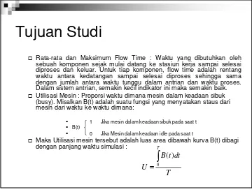
Rata-rata dan Maksimum Flow Time : Waktu yang dibutuhkan oleh
b
h k
j k
l i d t
k
t
i
k j
i
l
i
sebuah komponen sejak mulai datang ke stasiun kerja sampai selesai
diproses dan keluar. Untuk tiap komponen, flow time adalah rentang
waktu antara kedatangan sampai selesai diproses sehingga sama
dengan jumlah antara waktu tunggu dalam antrian dan waktu proses.
Dalam sistem antrian, semakin kecil indikator ini maka semakin baik.
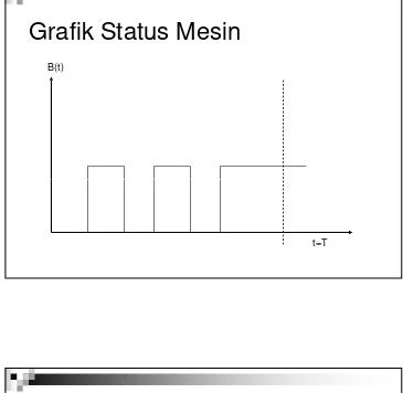
Utilisasi Mesin : Proporsi waktu dimana mesin dalam keadaan sibuk
(busy). Misalkan B(t) adalah suatu fungsi yang menyatakan staus dari
mesin dari waktu ke waktu dimana:
1 Jika mesin dalam keadaan sibuk pada saat t B(t)
0 Jika Mesin dalam keadaan idle pada saat t
Maka Utilisasi mesin tersebut adalah luas area dibawah kurva B(t) dibagi
dengan panjang waktu simulasi :
T
dt
t
B
U
T
0)
(
Grafik Jumlah Antrian
Grafik Status Mesin
B(t)
t=T
Waktu Kedatangan dan Proses
Satuan yang kita gunakan
Menit
Satuan yang kita gunakan
Menit
Pa r t N u m be r
Ar r iv a l Tim e
I n t e r va l Tim e
Se r v ice Tim e
1 0 . 0 0 6 . 8 4 4 . 5 8 2 6 . 8 4 2 . 4 0 2 . 9 6 3 9 . 2 4 2 . 7 0 5 . 8 6 4 1 1 . 9 4 2 . 5 9 3 . 2 1 5 1 4 . 5 3 0 . 7 3 3 . 1 1
Simulasi akan dilaksanakan selama 15
Kurva Q(t)
1 2 3
Q( t )
0 1 2 3 4 5 6 7 8 9 1 0 1 1 1 2 1 3 1 4 1 5
Kurva B(t)
1 2 3
B( t )
Event
Event
Menggambar keajadian yang baru terjadi.
Arr = Arrival, Dep= Departure
Variables
Q(t)
Jumlah
parts
yang antri dalam waktu t
B(t)
Server busy system
Attributes
If Part is in service at the machine, its arrival time is
underlined
Statistical Acumulators
P
= the total number of the parts produced so far
N
= the number of the entities that have passed throught the
queue so far
D = the sum of the queue times that have been observed so far
D* = the maximum time in queue observed so far
F
= the sum of the flowtimes that have been observed so far
F*
= the maximum flowtimes observed so far
= the area under the Q(t) curved so far
the area under the Q(t) curved so far
Q* = the maximum value of Q(t) so far
Simulation by Hand
Manually track state variables statistical
Manually track state variables, statistical
accumulators
Use “given” interarrival, service times
Keep track of event calendar
“Lurch” clock from one event to the next
Lurch clock from one event to the next
Will omit times in system, “max”
computations here (see text for complete
details)
System Clock B(t) Q(t) Arrival times of custs. in queue
Event calendar
Number of Total of Area under Area under
Simulation by Hand:
Setup
completed waiting times in queue
waiting times in queue Q(t) B(t)
Q(t) graph
0 1 2 3 4
0 5 10 15 20
2
B(t) graph
Time (Minutes)
Interarrival times 1.73, 1.35, 0.71, 0.62, 14.28, 0.70, 15.52, 3.15, 1.76, 1.00, ... 0
1 2
System Clock
0.00
B(t)
0
Q(t)
0
Arrival times of custs. in queue
<empty>
Event calendar [1, 0.00, Arr] [–, 20.00, End]
Number of Total of Area under Area under
Simulation by Hand:
t
= 0.00, Initialize
completed waiting times in queue 0
waiting times in queue
0.00
Q(t)
0.00
B(t)
0.00
Q(t) graph
0 1 2 3 4
0 5 10 15 20
2
B(t) graph
Time (Minutes)
Interarrival times 1.73, 1.35, 0.71, 0.62, 14.28, 0.70, 15.52, 3.15, 1.76, 1.00, ... Service times 2.90, 1.76, 3.39, 4.52, 4.46, 4.36, 2.07, 3.36, 2.37, 5.38, ...
0 1 2
0 5 10 15 20
System Clock
0.00
B(t)
1
Q(t)
0
Arrival times of custs. in queue
<empty>
Event calendar [2, 1.73, Arr] [1, 2.90, Dep] [–, 20.00, End] Number of Total of Area under Area under
Simulation by Hand:
t
= 0.00, Arrival of Part 1
1
completed waiting times in queue 1
waiting times in queue
0.00
Q(t)
0.00
B(t)
0.00
Q(t) graph
0 1 2 3 4
0 5 10 15 20
2
B(t) graph
Time (Minutes)
Interarrival times 1.73, 1.35, 0.71, 0.62, 14.28, 0.70, 15.52, 3.15, 1.76, 1.00, ... Service times 2.90, 1.76, 3.39, 4.52, 4.46, 4.36, 2.07, 3.36, 2.37, 5.38, ...
0 1 2
System Clock
1.73
B(t)
1
Q(t)
1
Arrival times of custs. in queue
(1.73)
Event calendar [1, 2.90, Dep] [3, 3.08, Arr] [–, 20.00, End] Number of Total of Area under Area under
Simulation by Hand:
t
= 1.73, Arrival of Part 2
1
2
completed waiting times in queue 1
waiting times in queue
0.00
Q(t)
0.00
B(t)
1.73
Q(t) graph
0 1 2 3 4
0 5 10 15 20
2
B(t) graph
Time (Minutes)
Interarrival times 1.73, 1.35, 0.71, 0.62, 14.28, 0.70, 15.52, 3.15, 1.76, 1.00, ... Service times 2.90, 1.76, 3.39, 4.52, 4.46, 4.36, 2.07, 3.36, 2.37, 5.38, ...
0 1 2
0 5 10 15 20
System Clock
2.90
B(t)
1
Q(t)
0
Arrival times of custs. in queue
<empty>
Event calendar [3, 3.08, Arr] [2, 4.66, Dep] [–, 20.00, End] Number of Total of Area under Area under
Simulation by Hand:
t
= 2.90, Departure of Part 1
2
completed waiting times in queue 2
waiting times in queue
1.17
Q(t)
1.17
B(t)
2.90
Q(t) graph
0 1 2 3 4
0 5 10 15 20
2
B(t) graph
Time (Minutes)
Interarrival times 1.73, 1.35, 0.71, 0.62, 14.28, 0.70, 15.52, 3.15, 1.76, 1.00, ... 0
1 2
System Clock
3.08
B(t)
1
Q(t)
1
Arrival times of custs. in queue
(3.08)
Event calendar [4, 3.79, Arr] [2, 4.66, Dep] [–, 20.00, End] Number of Total of Area under Area under
Simulation by Hand:
t
= 3.08, Arrival of Part 3
2
3
completed waiting times in queue 2
waiting times in queue
1.17
Q(t)
1.17
B(t)
3.08
Q(t) graph
0 1 2 3 4
0 5 10 15 20
2
B(t) graph
Time (Minutes)
Interarrival times 1.73, 1.35, 0.71, 0.62, 14.28, 0.70, 15.52, 3.15, 1.76, 1.00, ... Service times 2.90, 1.76, 3.39, 4.52, 4.46, 4.36, 2.07, 3.36, 2.37, 5.38, ...
0 1 2
0 5 10 15 20
System Clock
3.79
B(t)
1
Q(t)
2
Arrival times of custs. in queue
(3.79, 3.08)
Event calendar [5, 4.41, Arr] [2, 4.66, Dep] [–, 20.00, End] Number of Total of Area under Area under
Simulation by Hand:
t
= 3.79, Arrival of Part 4
2
3
4
completed waiting times in queue 2
waiting times in queue
1.17
Q(t)
1.88
B(t)
3.79
Q(t) graph
0 1 2 3 4
0 5 10 15 20
2
B(t) graph
Time (Minutes)
Interarrival times 1.73, 1.35, 0.71, 0.62, 14.28, 0.70, 15.52, 3.15, 1.76, 1.00, ... Service times 2.90, 1.76, 3.39, 4.52, 4.46, 4.36, 2.07, 3.36, 2.37, 5.38, ...
0 1 2
System Clock
4.41
B(t)
1
Q(t)
3
Arrival times of custs. in queue
(4.41, 3.79, 3.08)
Event calendar [2, 4.66, Dep] [6, 18.69, Arr] [–, 20.00, End] Number of Total of Area under Area under
Simulation by Hand:
t
= 4.41, Arrival of Part 5
2
3
4
5
completed waiting times in queue 2
waiting times in queue
1.17
Q(t)
3.12
B(t)
4.41
Q(t) graph
0 1 2 3 4
0 5 10 15 20
2
B(t) graph
Time (Minutes)
Interarrival times 1.73, 1.35, 0.71, 0.62, 14.28, 0.70, 15.52, 3.15, 1.76, 1.00, ... Service times 2.90, 1.76, 3.39, 4.52, 4.46, 4.36, 2.07, 3.36, 2.37, 5.38, ...
0 1 2
0 5 10 15 20
System Clock
4.66
B(t)
1
Q(t)
2
Arrival times of custs. in queue
(4.41, 3.79)
Event calendar [3, 8.05, Dep] [6, 18.69, Arr] [–, 20.00, End] Number of Total of Area under Area under
Simulation by Hand:
t
= 4.66, Departure of Part 2
3
4
5
completed waiting times in queue 3
waiting times in queue
2.75
Q(t)
3.87
B(t)
4.66
Q(t) graph
0 1 2 3 4
0 5 10 15 20
2
B(t) graph
Time (Minutes)
Interarrival times 1.73, 1.35, 0.71, 0.62, 14.28, 0.70, 15.52, 3.15, 1.76, 1.00, ... 0
1 2
System Clock
8.05
B(t)
1
Q(t)
1
Arrival times of custs. in queue
(4.41)
Event calendar [4, 12.57, Dep] [6, 18.69, Arr] [–, 20.00, End] Number of Total of Area under Area under
Simulation by Hand:
t
= 8.05, Departure of Part 3
4
5
completed waiting times in queue 4
waiting times in queue
7.01
Q(t)
10.65
B(t)
8.05
Q(t) graph
0 1 2 3 4
0 5 10 15 20
2
B(t) graph
Time (Minutes)
Interarrival times 1.73, 1.35, 0.71, 0.62, 14.28, 0.70, 15.52, 3.15, 1.76, 1.00, ... Service times 2.90, 1.76, 3.39, 4.52, 4.46, 4.36, 2.07, 3.36, 2.37, 5.38, ...
0 1 2
0 5 10 15 20
System Clock
12.57
B(t)
1
Q(t)
0
Arrival times of custs. in queue
()
Event calendar [5, 17.03, Dep] [6, 18.69, Arr] [–, 20.00, End] Number of Total of Area under Area under
Simulation by Hand:
t
= 12.57, Departure of Part 4
5
completed waiting times in queue 5
waiting times in queue
15.17
Q(t)
15.17
B(t)
12.57
Q(t) graph
0 1 2 3 4
0 5 10 15 20
2
B(t) graph
Time (Minutes)
Interarrival times 1.73, 1.35, 0.71, 0.62, 14.28, 0.70, 15.52, 3.15, 1.76, 1.00, ... Service times 2.90, 1.76, 3.39, 4.52, 4.46, 4.36, 2.07, 3.36, 2.37, 5.38, ...
0 1 2
System Clock
17.03
B(t)
0
Q(t)
0
Arrival times of custs. in queue ()
Event calendar [6, 18.69, Arr] [–, 20.00, End]
Number of Total of Area under Area under
Simulation by Hand:
t
= 17.03, Departure of Part 5
completed waiting times in queue 5
waiting times in queue
15.17
Q(t)
15.17
B(t)
17.03
Q(t) graph
0 1 2 3 4
0 5 10 15 20
2
B(t) graph
Time (Minutes)
Interarrival times 1.73, 1.35, 0.71, 0.62, 14.28, 0.70, 15.52, 3.15, 1.76, 1.00, ... Service times 2.90, 1.76, 3.39, 4.52, 4.46, 4.36, 2.07, 3.36, 2.37, 5.38, ...
0 1 2
0 5 10 15 20
System Clock
18.69
B(t)
1
Q(t)
0
Arrival times of custs. in queue ()
Event calendar [7, 19.39, Arr] [–, 20.00, End] [6, 23.05, Dep] Number of Total of Area under Area under
Simulation by Hand:
t
= 18.69, Arrival of Part 6
6
completed waiting times in queue 6
waiting times in queue
15.17
Q(t)
15.17
B(t)
17.03
Q(t) graph
0 1 2 3 4
0 5 10 15 20
2
B(t) graph
Time (Minutes)
Interarrival times 1.73, 1.35, 0.71, 0.62, 14.28, 0.70, 15.52, 3.15, 1.76, 1.00, ... 0
1 2
System Clock
19.39
B(t)
1
Q(t)
1
Arrival times of custs. in queue
(19.39)
Event calendar [–, 20.00, End] [6, 23.05, Dep] [8, 34.91, Arr] Number of Total of Area under Area under
Simulation by Hand:
t
= 19.39, Arrival of Part 7
6
7
completed waiting times in queue 6
waiting times in queue
15.17
Q(t)
15.17
B(t)
17.73
Q(t) graph
0 1 2 3 4
0 5 10 15 20
2
B(t) graph
Time (Minutes)
Interarrival times 1.73, 1.35, 0.71, 0.62, 14.28, 0.70, 15.52, 3.15, 1.76, 1.00, ... Service times 2.90, 1.76, 3.39, 4.52, 4.46, 4.36, 2.07, 3.36, 2.37, 5.38, ...
0 1 2
0 5 10 15 20
Simulation by Hand:
t
= 20.00, The End
6
7
System Clock
20.00
B(t)
1
Q(t)
1
Arrival times of custs. in queue
(19.39)
Event calendar [6, 23.05, Dep] [8, 34.91, Arr]
Number of Total of Area under Area under
0 1 2 3 4
0 5 10 15 20
2 completed waiting times in queue 6
waiting times in queue
15.17
Q(t)
15.78
B(t)
18.34
Q(t) graph
0 1 2
0 5 10 15 20
B(t) graph
Time (Minutes)
Simulation by Hand:
Finishing Up
Average waiting time in queue:
17
15
i
ti
f
T t l
Time-average number in queue:
part
per
minutes
53
2
6
17
15
queue
in
times
of
No.
queue
in
times
of
Total
.
.
part
79
0
20
78
15
l
l
k
Fi
l
curve
under
Area
.
.
)
(
t
Q
Utilization of drill press:
p
20
value
clock
Final
less)
(dimension
92
0
20
34
18
value
clock
Final
curve
under
Area
.
.
)
(
t
B
Tugas
Buatlah kembali grafik B(t) dan Q(t) dalam
Buatlah kembali grafik B(t) dan Q(t) dalam