6
and Forecasting
C O N C E P T S
● Regression Method ● Scatter Diagram
● Linear Regression ● Regression Line
● Independent Variable ● Explanatory Variable
● Dependent Variable ● Intercept Coefficient
● Slope Coefficient ● Least-Squares Estimates
● Simple Regression ● Multiple Regression
● Demand Forecasting ● Short-term Forecasting
● Medium-term Forecasting ● Long-term Forecasting
● Expert Opinion ● Delphi Method
● Consumer Polls and Surveys ● Time Series Analysis
● Time Series Plot/Graph ● Trend Component
● Seasonal Component ● Cyclical Component
● Randomness or Error ● De-seasonlising
W
e have learnt about how various factors like own price, prices of related goods and income affect the demand for a particular commodity or service. The demand function introduced in Chapter 2 is a symbolic (mathematical) expression of such cause-effect relationships. However, what is the exact (quantitative) relationship, say, between own price and quantity demanded of a product in an actualmarket situation? For instance, what is the exact shape and position of the household demand curve for electricity in the state of Karnataka? What does the demand curve for petrol look like for the whole of India?It is very useful to know the quantitative nature of a demand curve because, if we know it, we can compute various elasticities like price elasticity and income elasticity. In Chapter 2, we have already discussed the potential applications of elasticities in managerial, business and other environments. Essentially, elastici-ties can be utilised to predict demand or changes in demand, based on assump-tions about prices, income and so on as well as the changes in these. One of the objectives in this chapter is to briefly outline the procedure of ‘estimating’ or quantifying a demand function by using data on quantity demanded, prices and income and so on.
In a business environment, in particular, the forecasting of demand is quite important. A steel manufacturer in India would be interested to obtain a forecast-ing on the demand for steel in India, given the extent of competition from imports of steel from Korea and other countries. To make production plans, Maruti Udyog should be interested in the forecasting of demand for autos in the next few years to come. Forecasting is important not just at the national level but also at a local or regional level in deciding, for example, whether to open a local or regional office. In this chapter, we study demand forecasting as well.
DEMAND ESTIMATION BY REGRESSION METHOD
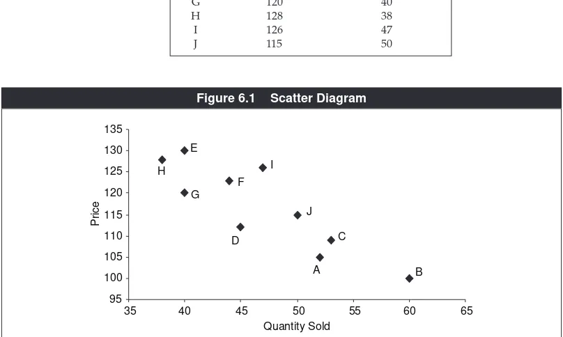
Suppose that a local small-scale garment company makes jeans of its own unique brand and sells these in various outlets in several cities. The general sales manager of this company has collected data from different outlets on the price charged and the number of jeans sold of its brand in a month. This is given in Table 6.1.
The various price–quantity combinations are plotted in Figure 6.1, which is a
scatter diagram, generally defined as the plot of data on various combinations of
two variables. Here the two variables are price and quantity sold. This diagram indicates the nature of the relationship between the two variables. For instance, Figure 6.1 roughly tells that lower prices are associated with higher quantities demanded, that is, the relationship between quantity demanded and the own price is negative.
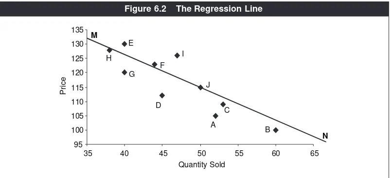
The regression analysis typically assumes a straight line relationship between the two variables involved. If so, it is called linear regression. Thus, in our example, assuming linear regression, we look for a straight line that best represents the points A, B, C, …, J. In Figure 6.2, MN is shown to represent this line, and it is the estimated demand function. In terms of regression, MN is called the regression line.
More exactly and algebraically, suppose that we want to estimate the effect of a variable Xon another variable Y. In the regression analysis, Xis then the
inde-pendentor the explanatory variableand Ythe dependent variable, meaning that
the changes in Xgovern the changes in Ynot but vice versa. For example, in
esti-mating a demand function, X will be the own price and Y will be quantity
sold/demanded since a demand relationship describes how a change in price affects a change in the quantity sold.
Let the various observations in the data on X and Y be denoted as (X 1, Y1),
(X
2,Y2) and so on. In our example, in Table 6.1, (X1, Y1), (X2, Y2) and so on refer to Table 6.1 Price–Quantity Sold Data
Outlet Price (Rs) Number of Jeans Sold
entries A, B, C, ... up to J. Next, let the assumed straight line or the linear relation-ship between Xand Ybe generally stated as:
Y=a + bX,
where aand bare constants; typically ais called the intercept coefficientand b (the multiplicative term with the independent variable) is called the slope coefficient.1
The regression analysis estimates these coefficients a and b and this completely defines the linear regression equation.
Intuitively, you can see that the regression line must be the one that passes through the scatter points such that its ‘aggregate distance,’ in some sense, from these points is minimised. More precisely, aand bare chosen such that the sum of the squares of the distance, along the axis measuring the dependent variable, between the scatter points and the regression line is minimised. This is why the estimates of aand bare called the least-squares estimates.
There are interpretations of aand b. Since bis the coefficient of X,its magnitude and sign capture the marginal effect of the explanatory variable Xon Y. However,
Ymay also be affected by factors other than X. The coefficient arepresents the effects of other possible explanatory variables outside of the regression analysis.
In our example given in Table 6.1, the regression or the least-squares estimates turn out to be a=115.645 and b= −0.588.2Note that bis negative, reflecting a
neg-ative relationship between the price and the quantity demanded, as can be visu-ally inspected in Figure 6.1. If, instead, we obtained a scatter diagram for a
1This is because if we graph X and Y respectively on the x-axis and y-axis, a is the intercept on the y-axis and b is the slope
of the line.
2Any standard textbook on statistics will have the least-squares formulae for computing a and b.
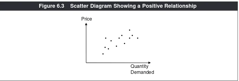
demand relationship as shown in Figure 6.3, bwould be positive, indicating the case of a Giffen good. In general, in the regression analysis, a positive or a nega-tive relation between two variables will lead to a slope coefficient having a posi-tive or negaposi-tive sign respecposi-tively.
In the above, we have described what is called a simple regression, defined as one that has one explanatory variable. More desirably, in estimating a relationship, other relevant explanatory variables should be included—for example, the con-sumers’ income, the prices of related goods and so on—in estimating a demand function. Of course, which variables are included in practice depends on the avail-ability of data. In any case, in principle when more than one explanatory variable is included in a regression, it is called multiple regression.
Algebraically, let there be nexplanatory variables available, namely, X
1, X2, ..., Xn.
Then a multiple, linear regression can be stated as:
Y=a + b
1X1+b2X2+ … + bnXn,
where b
1captures the marginal effect of X1on Y,b2 captures the marginal effect of
X
2on Yand so on. The task is to estimate a, b1, b2, et cetera.
Although multiple regression is more complicated, the general principle behind it is the same as that of simple regression. The idea is to choose the vari-ous coefficients such that the regression equation best fits the data points.
In summary then the regression analysis has the following elements:
(a) It requires data on the dependent variable and some of the explanatory variables.
(b) A mathematical equation describing the relationship between the depend-ent variable and the available explanatory variables is postulated. Typically, a linear relationship is assumed. If so, it is called linear regression.
(c) In the linear regression, the intercept coefficient and the slope coefficients are estimated on the criterion that the sum of squares of the difference between the actual values of the dependent variable and its values according to the
• •
• •
• • •
• • •
•
• •
Quantity Demanded Price
regression equation is minimised (In simple regression, it reduces to the sum of squares of the distance, along the axis measuring the dependent variable, between the scatter points and the regression line.) Such estimates of the coefficients are called the least-squares estimates.
(d) The sign and the magnitude of a slope coefficient show the sign and
mag-nitude of the marginal effect of the corresponding explanatory variable on the dependent variable. In case of a demand estimation, the slope coefficient of the own price should turn out to be negative (unless it is a Giffen good).
Does the regression method give a ‘perfect’ estimation of what the true rela-tionship (for example, demand relarela-tionship) is? The answer is no and never. However, there is a general question of how good a fit the regression line is in relation to the data. That depends on the explanatory variables chosen (based on available data) as well as variations in the values of the explanatory variables. For example, if a relevant explanatory variable is missing (due to data problems or because it has not occurred to the researcher that the particular variable is per-tinent), then the fit will be poor. This does not, however, mean that regression is a bad method. (Do not lose sight of the fact that nothing is perfect.) If the fit of the regression equation is good (and there are statistical measures to estimate what is called the ‘goodness of fit’), then regression estimates can be considered reliable.
DEMAND FORECASTING
Earlier, we gave examples of how demand forecasting can be useful to managerial decision-making within a firm. It can also be useful for the government in policy making. For example, a forecasting on the demand for petrol may guide the gov-ernment’s policy toward petrol pricing, building of reserves and so on. A good demand forecasting for HIV vaccine is considered to be important for developing countries where AIDS is a growing phenomenon.
There are different kinds of demand forecasting depending on (a) the time
hori-zon and (b) the method involved. In the business world, quantity decisions that
ought to change periodically in response to demand will benefit from a short-run forecasting. Examples include forecasting on inventory demand and demand for various raw materials. As a rough approximation, a forecasting up to six months ahead can be regarded as a short-term forecasting. Amedium-term forecasting
on demand (say 2–3 years hence) will be useful for decisions like a plant expan-sion or contraction and entering a new market. Along-term demand forecasting, over say 5 years, will be critical in decision-making such as setting up of R&D (research and development) infrastructure for the introduction of a new product or product line or setting up a new major plant.
There exist various demand forecasting techniques or methods. In what follows, we will discuss three of them: expert opinion, consumer polls and surveys, and time series analysis.
Expert Opinion
Many businesses often rely on expert opinion. Experts are presumably knowledge-able about the pattern of demand for certain products or industry in a certain region. In giving an opinion, an expert may use his intuition only or some data analysis. If the manager who seeks the forecasts is constrained to obtain one expert opinion, then that expert’s opinion is most likely the forecast to be used by the manager.
But a manager may be in a position to ask more than one expert. Suppose dif-ferent experts give very difdif-ferent opinions. How does the manager use this information? There is something called a Delphi techniquethat can be used—it essentially involves asking the experts repeatedly. It can be understood through a simple example. Suppose that there are three experts A, B and C. Over the next five years, according to A, the market demand for a product will grow at 10 per cent. B says that this growth rate will be 0, while C thinks that the market will grow at 6 per cent. There are thus huge differences in the expert opinion. Delphi method involves asking each expert again to submit revised estimates by pro-viding him what others have predicted. For instance, A will be told that the two other experts have projected the growth rate at 0 per cent and 6 per cent. Given a chance to reevaluate, A may lower his projection taking into account what oth-ers have said. Similarly C may revise his projection upwards. Suppose that in the next round, the numbers obtained are 7 per cent, 4 per cent and 5 per cent. These numbers are closer to each other than the earlier numbers. This technique involves obtaining reevaluations until the opinions converge or nearly con-verge. In the current example, a manager may think that the numbers 7, 4 and 5 are close enough for the purpose and he may decide the number say 5 or 5.5 (something very close to the average). Or the manager may decide to go for one more round.
There are, however, problems with the Delphi method. First, good experts are typically very busy people and their fees are very high. This may be a major con-straint for a manager. Second, it is not necessary that experts may want to revise their estimates. Because if they do it frequently, it may reflect that they are not very confident about themselves and, thus, that they do not possess a high expert-ise. They may not wish to hamper their reputation.
Despite these limitations, expert opinions on forecasts are much sought after in businesses.
Consumer Polls and Surveys
an annual survey called Market Information Survey of Households (MISH). A sample of 3 lakh households is used covering all districts in India. The survey asks the households about their income and their purchase of various products, both durable and non-durable, among other things. As the website of the NCAER indicates, this survey data is used, among others, by businesses like Bajaj Auto, Godrej and Bank of America.
There are market research companies which conduct consumer polls and surveys on specific products and sell their forecasting to their clients.
Time Series Analysis
It is a statistical method. In regression, the dependent variable (for example, quan-tity demanded of a product) is estimated on the basis of how it is influenced by ‘other factors’ or independent variables (for example, own price, consumers’ income). In the time series method, the idea is not to emphasise the relationship of one variable to some others, but to rely on the existing behaviour of the vari-able itself over time and extrapolate from that the likely future values of the variable.
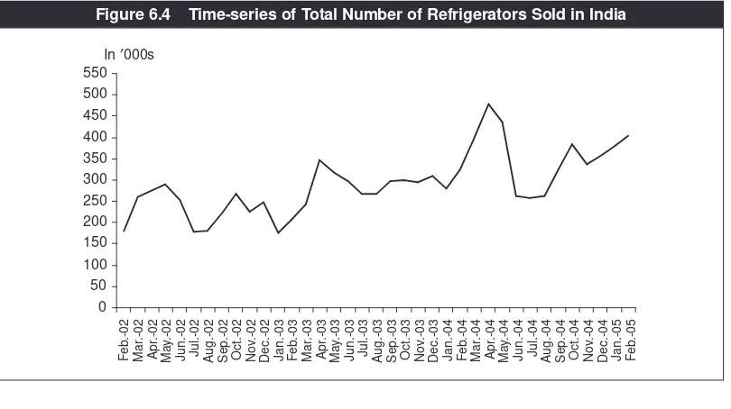
The existing pattern of change in a variable over time can be seen from a time series plot orgraph, which measures calendar time along the x-axis and the vari-able itself on the y-axis. For instance, Figure 6.4 shows the time series plot of monthly data on the number of refrigerators sold/consumed in India.3
0
Figure 6.4 Time-series of Total Number of Refrigerators Sold in India
In general, let time be denoted by t. Suppose that we have data on variableY
(for example, quantity demanded of a product) for t=0, 1, 2, …, T. The question
is: what is the forecast of Xfor t=T +1,T +2 and so on.
The time series analysis assumes that the value that a variable takes at any given point of time has four components.
One is a trendcomponent, capturing any long-run trend of growth or decline in the variable over time. For instance, if we have a time series plot of the total number of cell phones sold in India in the recent years, we are certain to see an upward, that is, a positive trend. But if we look at the total number of 14-inch black and white TV sets sold, we expect to see a negative trend.
Another in the seasonalcomponent. For many products and services, all other things remaining the same, the quantity demanded depends on the prevailing season. If we consider the demand for bottled mineral water, the demand is much higher in the summer than in the winter months. The demand for visits to general physicians for common sickness like cold, cough and flu is higher in the winter than in the summer months. Refrigerator sales are likely to reach their peak in months approaching or during summer. Indeed, Figure 6.4 shows that the sales are generally very high during March, April and May as compared to other months.
The third component is cyclical, relating to business-cycle reasons. For exam-ple, if the economy is passing through a recession, the demand for real estate is typically slack.
The last component is randomnessor errorresulting from unanticipated and unexplained events.
If we denote these four components respectively by T, S, Cand R, then the time
series analysis typically postulates:
Y=T’ S’ C’ R.
Forecasting involves methods which first attempt to neutralise the seasonal com-ponent by various averaging methods (that is, smoothing techniques). It is called
de-seasonalisingthe data, which essentially smoothens the data. Many computer
softwares are available that de-seasonalise a time series data.
Once the data is de-seasonalised, there are several methods available to filter out the T(trend) and the C(cyclical) components separately or jointly. Whatever left is,
by definition, the R(random) component.
The forecasting obtained in an actual situation depends on the sophistication of the methodology used, tools, computer software, time available and, not to men-tion, the skill of the individual entrusted with the task of forecasting.
As an illustration, a very simplistic procedure will involve fitting a linear trend line to a de-seasonalised time series data by the regression method and then extrapolating from it to a future date. That is, a regression equation of the form Y= a + btis assumed, where tdenotes calendar time (the independent
vari-able) and Y is a de-seasonalised variable under consideration (for example,
quantity demanded of a product). Using the least-squares estimates of aand b,
we can set tto any future date (for example, month or quarter) and compute the
Economic Facts and Insights
● The scatter diagram indicates the nature of relationship between two variables. ● In the regression method, a demand function is estimated by using data on
quantity demanded of a product and its determinants such as own price, prices of related goods and income.
● Under linear regression, the slope coefficient measures the marginal effect of
the respective explanatory variable on the dependent variable.
● If the slope coefficient is positive (or negative), it indicates a positive (or
neg-ative) relationship between the independent variable and the dependent variable.
● The intercept coefficient estimates the effect of other variables not included
in the regression.
● The regression method does not yield the perfect estimation of the true
rela-tionship between the dependent variable and the set of independent variables.
● Demand forecasting is achieved by soliciting expert opinion, using consumer
polls and surveys or by using time series techniques.
● In the time series method, the idea is not to emphasise the relationship of
one variable to some others, but to rely on the existing behaviour of the vari-able itself over time and extrapolate from that the likely future values of the variable.
● In the time series method, the data is de-seasonalised (by using smoothing
techniques) before the trend or the cyclical component is extracted.
● Linear trend line is obtained by regressing the de-seasonalised time series
data with respect to time.
E
E X
X E
E R
R C
C II S
S E
E S
S
6.1 Consider the following scatter diagram. If a regression line is fitted to this data, would it be positively sloped or negatively sloped? Explain.
• • •
• •
• •
•
• •
•
• •