SOME QUALITATIVE FEATURES OF 2D PERIODIC MIXING MODEL
Adela Ionescu, Mihai Costescu
Abstract. The problems of flow kinematics are far from complete solv-ing. Recently, the mixing theory issued in this field, with the mathematical methods and techniques, developed the significant relation between turbu-lence and chaos. The turbuturbu-lence is an important feature of dynamic systems with few freedom degrees, the so-called “far from equilibrium systems”, which are widespread between the models of excitable media.
In the previous works, the study of the 3D non-periodic models exhibited a quite complicated behavior. In agreement with experiments, they involved some significant events - the so-called “rare events”. The variation of param-eters had a great influence on the length and surface deformations.
The 2D (periodic) case is simpler, but significant events can issue for irrational values of the length and surface versors, as is the situation in 3D case. Also, the graphic analysis previously realized involved that in 2D case, the mixing has also a nonlinear behavior and the rare events can appear.
In this paper is started a computational analysis for 2D basic mixing model, in a modified version. In the first stage, there is analyzed the length deformation for different values of the basic parameters. For the simulations there are used specific procedures and functions of MapleVI. The conclusions will be further used for analyzing the mixing efficiency.
2000 Mathematics Subject Classification: 76F25, 37E35
1.Introduction
In the turbulence theory, two important fields are distinguished:
a) The transition theory from smooth laminar flows to chaotic flows, characteristic to turbulence.
From statistical standpoint, a flow is represented by the map:
x= Φt(X), X = Φt(t= 0) (X) (1)
which must be of class Ck. From the dynamic standpoint the map:
Φt(X)−→x (2)
is a diffeomorphism of class Ck and (1) must satisfy the relation
0< J <∞, J = det
∂xi
∂Xj
, J =det(DΦt(X)) (3)
where D denotes the derivation with respect to the reference configuration, in this case X. The relation (3) implies two particles, X1 and X2, which occupy the same position x at a moment. Non-topological behavior (like break up, for example) is not allowed.
With respect to X it is defined the basic measure for the deformation, namely the deformation gradient, F:
F= (∇XΦt(X))T , Fij =
∂xi
∂Xj
, or F=DΦt(X) (4)
where ∇X denotes differentiation with respect to X. According to (3), F is
non singular. The basic measure for the deformation with respect to x is the
velocity gradient ( ∇x denote differentiation with respect to x).
By differentiation ofxwith respect toX there are obtained the basic de-formation for a material filament, and for the area of an infinitesimal material surface [4].
Let us focus on the basic deformation measures:the length deformation λ and surface deformation η , with the relations [4,5]:
λ = (C :M M)12 , η= (detF)· C−1 :N N
1 2
, (5)
with C = FTF the Cauchy-Green deformation tensor, and the length and surface vectors M, N defined by
λ=Cij ·Mi·Nj, η = (detF)· Cij−1·Ni·Nj
, (7)
with P M2
i = 1,
P N2
j = 1.
The deformation tensor F and the associated tensors C, C−1 represent
the basic quantities in the deformation analysis for the infinitesimal elements. In this framework, the mixing concept implies the stretching and folding of the material elements. If in an initial locationP there is a material filament dX and an area element dA, the specific length and surface deformations are given by the relations:
D(lnλ)
Dt =D:mm,
D(lnη)
Dt =∇v−D :nn (8) where D is the deformation tensor, obtained by decomposing the velocity gradient in its symmetric and non-symmetric part [5]:
∇v=D+Ω
D =
∇v+ (∇v)T
2 the symmetric tensor (9)
Ω=
∇v−(∇v)T
2 the antisimetric tensor 2. The perturbed 2D mixing model. Results
Studying a mixing for a flow implies the analysis of successive stretching
and folding phenomena for its particles, the influence of parameters and initial conditions [6]. In the previous works, the study of the 3D non-periodic models exhibited a quite complicated behavior [1]. For the moment the aim is to study the behavior of the length deformation of the modified 2D mixing model, for some irrational values of the length versor, in order to search some significant events, and compare to 3D case.
Let us start from the basic (widespread) 2D mixing model [5]:
˙
x1 =G·x2 ˙
and consider a little perturbation of it, namely:
˙
x1 =G·x2+x1 ˙
x2 =K·G·x1+x2 (10) with −1< K <1, 0< G < 1.
Here is the time derivative. If we attach the initial condition:
x1(0) =X1, x2(0) =X2 (11)
the Cauchy problem (10)-(11) has the following calculated solution [3]:
x1 = "
X2 2 ·
P −√P KG − X1 2 · P √
P + 1 #
·exp1−√Pt+
" X1 2 · P √
P + 1
− X2 2 ·
(P −1)·√P KG
#
·exp1 +√Pt (12) and x2 = X2 2 − X1 2 · KG √ P
·exp1−√Pt+ X1 2 · KG √ P + X2 2 ·
1−√P
·exp1 +√P. (13)
Therefore, the deformation gradient (4) is found as:
F= −1 2 P √
P −1
·exp1−√Pt+ 1
2
P
√
P + 1
·exp1 +√Pt
1 2
P− √
P KG ·exp
1−√Pt− 1
2 (P−1)
√
P KG ·exp
1 +√Pt −12
KG
√
P ·exp
1−√Pt+ 1
2
KG
√
P ·exp
1 +√Pt
1 2exp
1−√Pt+ 1
2
1−√P·exp1 +√Pt (14) where 2 +KG2 not= P.
C=FT ·F
has the classical form,
C=
c11 c12 c21 c22
(15) with the notation
KG2 =γ (16)
and the components: c11 = γ
2
·(1+K)+γ·(5−2K)+6
4γK ·exp 1−
√ 2 +γ
2t+
γ3
+(K+2)·γ
2
+(1+7K)·γ+2
4γK ·exp 1 +
√ 2 +γ
2t− (K+1)·γ2+(K−3)·γ+6K+4
2γK ·exp (2t),
c12 = 14 ·
(−γ2−γ−2)· √
2+γ−4γ−4
γ(2+γ)
·exp 1−√2 +γ 2t+ 1
4 · h
(3γ+6)·√2+γ−2γ3−2γ2+3γ+2
γ(2+γ)
i
·exp (−1−γ)t+ 1
4 ·
(−2γ2−3γ−2)·√2+γ+2γ3+6γ2+3γ−2
γ(2+γ)
·exp 1 +√2 +γ 2t,
c21 = 14 ·
γ·(2+γ−√2+γ)
2+γ ·exp 1−
√ 2 +γ
2t+ 1
4 ·
γ·(2+γ+ √
2+γ)
2+γ ·exp 1 +
√ 2 +γ
2t− 14 ·2γ ·exp (−1−γ)t, c22 = 14 ·
γ2
2+γ + 1
·exp 1−√2 +γ 2t+ 1
4 · h
γ2
2+γ + 1 +
√
2 +γ2i·exp 1 +√2 +γ 2t+ 1
4 · h
−2+2γ2γ + 2 1−
√
2 +γi
·exp (−1−γ)t.
λ2 =
γ2
+5γ+6
4γ ·exp 1−
√ 2 +γ
2t+
γ3
+2γ2
+γ+2
4γ ·exp 1 +
√ 2 +γ
2t−
γ2
−3γ+4
2γ ·exp (2t)
·M
2 1+ 2
(−2γ
2
−γ−2)· √
2+γ+γ3
+2γ2
−4γ−4
γ(2+γ) ·exp 1− √
2 +γ 2t+ (−γ
2
−3γ−2)· √
2+γ+3γ3
+8γ2
+3γ−2
γ(2+γ) ·exp 1 + √
2 +γ 2t+ (3γ+6)·
√
2+γ−6γ2+3γ+2
γ(2+γ) ·exp (−1−γ)t
·
M1M2+
γ2
+γ+2
γ+2 ·exp 1− √
2 +γ 2t+
γ2
+(2+γ)(3+γ−2 √
2+γ)
2+γ ·exp 1 +
√ 2 +γ
2t+
−2γ2+(4+2γ)(1− √
2+γ)
2+γ ·exp (−1−γ)t
·
M22, (17)
where P M2
i = 1.
As it can be seen, the calculus is quite complex, some polynomials are involved for each exponential.
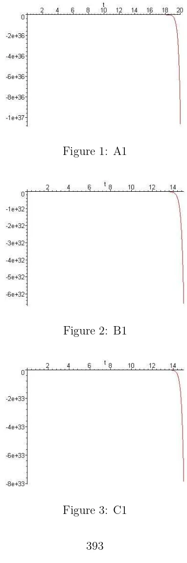
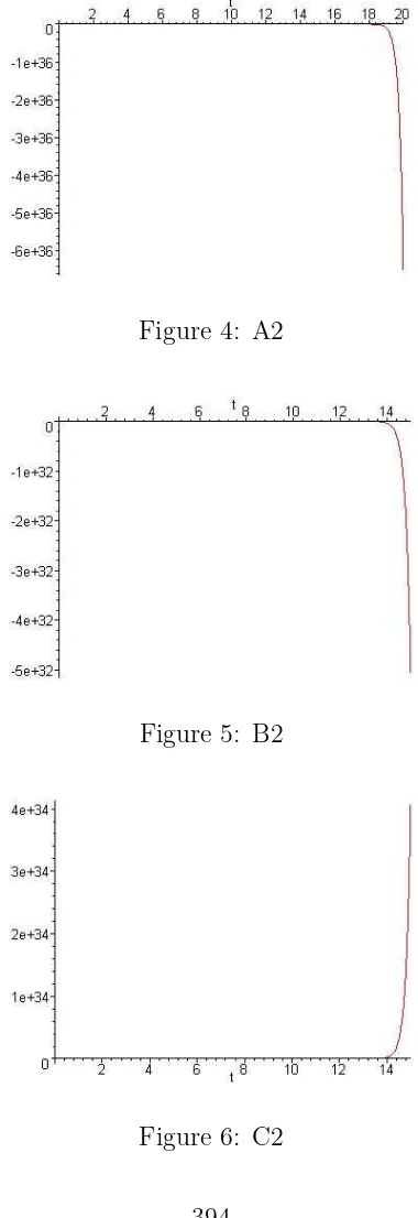
Let us consider two irrational, random, values for the length versor, namely:
(M1, M2) = −√1 3, √ 2 √ 3 ! ,
(M1, M2) = √1 7,−
√ 6 √ 7 ! .
For each of these cases, it is studied the behavior of the length deforma-tion, as function of time, for some values of γ. If we look at the relation (17), some symmetries of its form are observed. Therefore, taking into ac-count some remarks of [3], the following values of γ are taken into account, for the beginning:
A. γ =−0.75; B. γ =−0.05; C. γ = 0.75.
Figure 1: A1
Figure 2: B1
Figure 4: A2
[image:8.612.195.385.101.654.2]Figure 5: B2
3. Remarks
Looking at the above analysis, some remarks issue:
1. For any case of versor and/ or parameter case, the length deformation λ2 is unbounded. Moreover, for the first versor case, as γ increases, it must be shortened the axes, for avoiding the so-called “floating point overflow”, that means a breakup of the simulation. This happened also for the second versor case.
2. The length deformation has anegative behavior, although only a small time scale was considered. Only in the last case a positive behavior was noted. Thus, comparing to the cases studied in [1], it can be assessed that for a small perturbation of the 2D general model, and on a larger time interval, it becomes also far from equilibrium.
3. It can be assessed, as for 2D periodic case [2], that theirrational versor values produce nonlinear phenomena. It is expected that the efficiency of mixing has a more complicated expression.
4. As an immediate aim, more irrational versor values will be taken into account. That will be useful also for studying the efficiency of deformations, in length and also in surface. As perturbing the initial model, the calculus becomes very complex, therefore a parametric approach would be very useful. 5. The analysis of the length deformation for a small perturbation con-firms that the flows of the studied type, in 2D and 3D case, have a chaotic behavior. This matches the experiments in [6].
References
[1] Ionescu, A., The structural stability of biological oscillators. Analyti-cal contributions, Ph.D. Thesis. Politechnic University of Bucarest, 2002.
[2] Ionescu, A., Costescu, M. ”Computational aspects in excitable media. The case of vortex phenomena”. Proceedings of ICCCC2006, Oradea, ISSN 1841-1844, pag 280-284
[3] Ionescu, A., Costescu, M., Coman D. ”A computational approach of turbulent mixing. The trajectories analysis”. Proc. of ICEEMS2007, Brasov (in press)
[5] Ottino, J.M. ”The kinematics of mixing: stretching, chaos and trans-port”. Cambridge University Press. 1989, ISSN 0521368782
[6] Savulescu, St.N. ”Applications of multiple flows in a vortex tube closed at one end”. Internal Reports, CCTE, IEA. Bucarest. (1996-1998)
Authors:
Adela Ionescu
Department of Applied Sciences
Faculty of History, Philosophy and Geography University of Craiova
22 December 1989, No. 8, G5-III-3, 200724 Craiova e-mail: [email protected]
Mihai Costescu
Department of Political Sciences
Faculty of Engineering and Management of Technological Systems University of Craiova