El e c t ro n ic
Jo ur
n a l o
f P
r o
b a b il i t y
Vol. 13 (2008), Paper no. 50, pages 1380–1418. Journal URL
http://www.math.washington.edu/~ejpecp/
Large time asymptotics of growth models
on space-like paths I: PushASEP
Alexei Borodin
∗, Patrik L. Ferrari
†Abstract
We consider a new interacting particle system on the one-dimensional lattice that interpolates between TASEP and Toom’s model: A particle cannot jump to the right if the neighboring site is occupied, and when jumping to the left it simply pushes all the neighbors that block its way. We prove that for flat and step initial conditions, the large time fluctuations of the height function of the associated growth model along any space-like path are described by the Airy1and Airy2 processes. This includes fluctuations of the height profile for a fixed time and fluctuations of a tagged particle’s trajectory as special cases.
Key words:stochastic growth, KPZ, determinantal processes, Airy processes. AMS 2000 Subject Classification:Primary 82C22, 60K35, 15A52.
Submitted to EJP on August 30, 2007, final version accepted August 11, 2008.
∗California Institute of Technology, Mathematics 253-37, Pasadena, CA 91125, USA. E-mail: [email protected].
A. Borodin was partially supported by the NSF grants DMS-0402047 and DMS-0707163.
1
Introduction
We consider a model of interacting particle systems, which is a generalization of the TASEP (totally asymmetric simple exclusion process) and the Toom model. Besides the extension of some universal-ity results to a new model, the main feature of this paper is the extension of the range of analysis to any “space-like” paths in space-time, whose extreme cases are fixed time and fixed particle (tagged particle problem), see below for details.
Consider the system ofNparticles x1>· · ·>xN inZthat undergoes the following continuous time Markovian evolution: Each particle has two exponential clocks – one is responsible for its jumps to the left while the other one is responsible for its jumps to the right. All 2N clocks are independent, and the rates of all left clocks are equal toLwhile the rates of all right clocks are equal toR. When theith left clock rings, theith particle jumps to the nearest vacant site on its left. When theith right clock rings, theith particle jumps to the right by one provided that the sitexi+1 is empty; otherwise it stays put. The main goal of the paper is to study the asymptotic properties of this system when the number of particles and the evolution time become large.
IfL=0 then the dynamics is known under the name of Totally Asymmetric Simple Exclusion Process (TASEP), and ifR=0 the dynamics is a special case of Toom’s model studied in[9](see references therein too). Both systems belong to the Kardar-Parisi-Zhang (KPZ) universality class of growth models in 1+1 dimensions.
Particle’s jump to the nearest vacant spot on its left can be also viewed as the particle pushing all its left neighbors by one if they prevent it from jumping to the left. This point of view is often beneficial because it remains meaningful for infinite systems, and also the order of particles is not being changed. Because of this pushing effect we call our system the Pushing Asymmetric Simple Exclusion Process or PushASEP.
Observe that for a N-particle PushASEP with particles x1(t)>· · ·>xN(t), the evolution of
(x1, . . . ,xM) for any M ≤ N is the M-particle PushASEP not influenced by the presence of the
remainingN−M particles. This "triangularity property" seems to be a key feature of our model that allows our analysis to go through.
Our results split in two groups – algebraic and analytic.
Algebraically, we derive a determinantal formula for the distribution of the N-particle PushASEP with an arbitrary fixed initial condition, and we also represent this distribution as a gap probability for a (possibly, signed) determinantal point process (see [17; 12; 21; 16; 22] for information on determinantal processes). The result is obtained in greater generality with jump ratesLandRbeing both time and particle-dependent (Proposition 3.1). The first part (the determinantal formula, see Proposition 2.1) is a generalization of similar results due to[20; 19; 2]obtained by the Bethe Ansatz techniques. Also, a closely related result have been obtained very recently in[10]using a version of the Robinson-Schensted-Knuth correspondence.
Analytically, we use the above-mentioned determinantal process to study the large time behavior of the infinite-particle PushASEP with two initial conditions:
1. Flat initial condition with particles occupying all even integers.
2. Step initial condition with particles occupying all negative integers.
However, we take a simpler path here and consider our infinite-particle system as a limit of growing finite-particle systems. It turns out that for the above initial conditions, the distribution of any finite number of particles at any finitely many time moments stabilizes as the total number of particles in the system becomes large enough. It is this limiting distribution that we analyze.
We are able to control the asymptotic behavior of the joint distribution of xn1(t1), . . . ,xn
k(tk) with
xn1(0) ≥ · · · ≥ xnk(0)and t1 ≥ · · · ≥ tk. It is the second main novel feature of the present paper
(the first one being the model itself) that we can handle joint distributions of different particles at different time moments. As special cases we find distributions of several particles at a given time moment and distribution of one particle at several time moments (a.k.a. the tagged particle).
In the growth model formulation of PushASEP (that we do not give here; it can be easily recon-structed from the growth models for TASEP and Toom’s model described in [9] and references therein), this corresponds to joint distributions of values of the height function at a finite number of space-time points that lie on a space-like path; for that reason we use the term ‘space-like path’ below. The two extreme space-like paths were described above – they correspond to t1 =· · ·= tk
andn1=· · ·=nk.
The algebraic techniques of handling space-like paths are used in the subsequent paper [6]to an-alyze two different models, namely the polynuclear growth (PNG) model on a flat substrate and TASEP in discrete time with parallel update.
Our main result states that large time fluctuations of the particle positions along any space-like path have exponents 1/3 and 2/3, and that the limiting process is the Airy1 process for the flat initial condition and the Airy2 process for the step initial condition (see the review [11]and Section 2.4 below for the definition of these processes).
In the PushASEP model, we have the fluctuation exponent 1/3 even in the case of zero drift. This is due to the asymmetry in the dynamical rules and it is consistent with the KPZ hypothesis. In fact, from KPZ we expect to have the 1/3 exponent whenj′′(ρ)6=0, where j(ρ)is the current of particles as a function of their densityρ, and j′′(ρ) =−2(R+L/(1−ρ)3)for PushASEP.
We find it remarkable that up to scaling factors, the fluctuations are independent of the space-like path we choose (this phenomenon was also observed in[7]for the polynuclear growth model (PNG) with step initial condition). It is natural to conjecture that this type of universality holds at least as broadly as KPZ-universality does.
Interestingly enough, so far it is unknown how to study the joint distribution of xn1(t1)and xn2(t2) with xn1(0) > xn2(0)and t1 < t2 (two points on a time-like path); this question remains a major open problem of the subject.
Previous results. For the TASEP and PNG models, large time fluctuation results have already been obtained in the following cases: For the step initial condition the Airy2 process has been shown to occur in the scaling limit for fixed time[18; 14; 15], and more recently for tagged particle[13]. For TASEP, the Airy1process occurs for flat initial conditions in continuous time[4]and in discrete time with sequential update [3] with generalization to the initial condition of one particle everyd ≥2 sites1. Also, a transition between the Airy2and Airy1 processes was obtained in[5]. These are fixed time results; the only previous result concerning general space-like paths is to be found in[7]in the
context of the PNG model, where the Airy2process was obtained as a limit for a directed percolation model.
Outline. The paper is organized as follows. In Section 2 we describe the model and the results. In Proposition 2.1 the transition probability of the model is given. Then, we define what we mean by space-like paths, and formulate the scaling limit results; the definitions of the Airy1 and Airy2 processes are recalled in Section 2.4. In Section 3 we state the general kernel for PushASEP (Propo-sition 3.1) and then particularize it to step and flat initial conditions (Propo(Propo-sition 3.4 and 3.6). In Section 4 we first prove Proposition 2.1 and then obtain the general kernel for a determinantal mea-sure of a certain form (Theorem 4.2), which includes the one of PushASEP. Finally, the asymptotic analysis is the content of Section 5.
Acknowledgments
We are very grateful to the anonymous referee for careful reading and a number of constructive remarks. A.Borodin was partially supported by the NSF grants DMS-0402047 and DMS-0707163.
2
The PushASEP model and limit results
2.1
The PushASEP
The model we consider is an extension of the well known totally asymmetric simple exclusion pro-cess (TASEP) on Z. The allowed configuration are like in the TASEP, i.e., configurations consist of
particles onZ, with the constraint that at each site can be occupied by at most one particle
(exclu-sion constraint). We consider a dynamics in continuous time, where particles are allowed to jump to the right and to the left as follows. A particle jumps to its right-neighbor site with some rate, pro-vided the site is empty (TASEP dynamics). To the left, a particle jump to its left-neighbor site with some rate and, if the site is already occupied by another particle, this is pushed to its left-neighbor and so on (push dynamics).
To define precisely the jump rates, we need to introduce a few notations. Since the dynamics preserves the relative order of particles, we can associate to each particle a label. Let xk(t) be the position of particle k at time t. We choose the right-left labeling, i.e., xk(t)> xk+1(t) for all
k∈I⊆Z, t≥0. With this labeling, we considervk>0,k∈I, and some smooth positive increasing
functionsa(t),b(t)witha(0) =b(0) =0. Then, the right jump rate of particlekis ˙a(t)vk, while its left jump rate is ˙b(t)/vk.
In Proposition 2.1 we derive the expression of the transition probability from time t =0 to time t
forN particles, proven in Section 4.
Proposition 2.1. Consider N particles with initial conditions xi(0) = yi. Denote its transition proba-bility until time t by
G(xN, . . . ,x1;t) =P(x
Then
G(xN, . . . ,x1;t) (2.2)
= YN
n=1
vxn−yn
n e−
a(t)vne−b(t)/vn
detFk,l(xN+1−l−yN+1−k,a(t),b(t))
1≤k,l≤N,
where
Fk,l(x,a,b) =
1 2πi
I
Γ0 dzzx−1
Qk−1
i=1(1−vN+1−iz)
Ql−1
j=1(1−vN+1−jz)
ebzea/z, (2.3)
whereΓ0is any anticlockwise oriented simple loop with including only the pole at z=0.
2.2
Space-like paths
The computation of the joint distribution of particle positions at a given time t can be obtained from Proposition 2.1 by adapting the method used in[4]for the TASEP. However, one of the main motivation for this work is to enlarge the spectrum of the situations which can be analyzed to what we call space-like paths. In this context, space-like paths are sequences of particle numbers and times in the ensemble
S ={(nk,tk),k≥1|(nk,tk)≺(nk+1,tk+1)}, (2.4) where, by definition,
(ni,ti)≺(nj,tj)if nj≥ni,tj≤ti, and the two couples are not identical. (2.5)
The two extreme cases are (1) fixed time, tk = t for all k, and (2) fixed particle number, nk = n
for allk. This last situation is known as tagged particleproblem. Since the analysis is of the same degree of difficulty for any space-like path, we will consider the general situation.
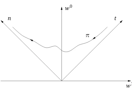
Consider any smooth functionπ,w0=π(w1), in the forward light cone of the origin that satisfies
|π′| ≤1, |w1| ≤π(w1). (2.6)
These are space-like paths inR×R+, see Figure 1. The first condition (the space-like property) is
related to the applicability of our result to sequences of particles inS. The second condition just reflects the choice of having t ≥0 and n≥ 0. Time and particle number are connected with the variablesw1 andw0by a rotation of 45 degrees. To avoid unnecessaryp2’s, we set
¨
w1 = t−2n w0 = t+n
2
«
⇐⇒
¨
t = w0+w1 n = w0−w1
«
(2.7)
We want to study the joint distributions of particle positions in the limit of large time, where uni-versal processes arise. Since we consider several times, we can not simply use t as large parameter. Instead, we consider a large parameterT. Particle numbers and times under investigation will have a leading term proportional to T. In the(w1,w0)plane, we considerw1 around θT for a fixedθ, while w0 =Tπ(w1/T). From KPZ we know that correlations are onT2/3 scale. Therefore, we set the scaling as (
w1(u) =θT−uT2/3,
n t w0
w1 π
Figure 1: An example of a space-like path. Its slope is, in absolute value, at most 1.
Notice thatw0(u) is equal to Tπ(w1(u)/T)up to terms that remain bounded, and they become ir-relevant in the largeTlimit, since the fluctuations grow asT1/3. Coming back to the(n,t)variables, we have
t(u) = (π(θ) +θ)T−(π′(θ) +1)uT2/3+1
2π
′′(θ)u2T1/3,
n(u) = (π(θ)−θ)T+ (1−π′(θ))uT2/3+12π′′(θ)u2T1/3. (2.9)
In particular, settingπ(θ) =1−θwe get the fixed time case witht=T, while settingπ(θ) =α+θ
we get the tagged particle situation with particle numbern=αT.
2.3
Scaling limits
Universality occurs in the largeT limit. In Proposition 3.1 we obtain an expression for the joint dis-tribution in the general setting. For the asymptotic analysis we consider the case where all particles have the same jump rates, i.e., we set
vk=1 for allk∈I. (2.10)
Moreover, we consider time-homogeneous case, i.e., we set a(t) = Rt and b(t) = L t for some
R,L≥0 (for time non-homogeneous case, one would just replaceRandLby some time-dependent functions). Two important initial conditions are
(a)flat initial condition: particles start from 2Z,
(b)step initial condition: particles start fromZ
−={. . . ,−3,−2,−1}.
In the first case, the macroscopic limit shape is flat, while in the second case it is curved, see[11]for a review on universality in the TASEP. For TASEP with step initial conditions and particle-dependent ratesvk, the study of tagged particle has been carried out in[13].
Flat initial conditions
wherevis the mean speed of particles, given by
v=−2L+R/2. (2.11)
The reason is that the density of particle is 1/2 and the particles jumps to the right with rate R
but the site on its right has a 1/2 chance to be empty. Moreover, particles move (and push) to the left with rate Lbut typically every second move to the left is due to a push from another particle. Therefore, the rescaled process is given by
u7→XT(u) =
xn(u)(t(u))−(−2n(u) +vt(u))
−T1/3 , (2.12)
where n(u) andt(u)are defined in (2.9). The rescaled processXT has a limit for largeT given in
terms of the Airy1 process,A1(see[4; 5; 11]and Section 2.4 for details onA1).
Theorem 2.2(Convergence to the Airy1process). Let us set the vertical and horizontal rescaling
Sv= ((8L+R)(π(θ) +θ))1/3, Sh=
4((8L+R)(π(θ) +θ))2/3
(R+4L)(π′(θ) +1) +4(1−π′(θ)). (2.13)
Then
lim
T→∞XT(u) =SvA1(u/Sh) (2.14)
in the sense of finite dimensional distributions.
The proof of this theorem is in Section 5. The specialization for fixed time t=T is
Sv= (8L+R)1/3, Sh= (8L+R)
2/3
2 , (2.15)
and the one for tagged particlen=αT at timest(u) =T−2uT2/3, obtained by settingθ= (1−α)/2, is
Sv= (8L+R)1/3, Sh= 2(8L+R)
2/3
4L+R . (2.16)
Step initial condition
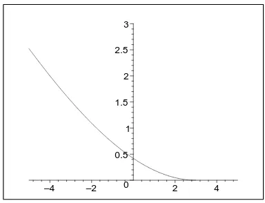
The proper rescaled process for step initial condition is quite intricate. Denote byβt the typical position of particle with number aroundαt at time t. In the situations previously studied in the literature, there was a nice functionβ=β(α). In the present situation this is not anymore true, but we can still describe the limit shape. More precisely,αandβare parametrized by aµ∈(0, 1)via
α(µ) = (1−µ)2(R+L/µ2), β(µ) =−((1−2µ)R+L/µ2). (2.17)
The parameterµcomes from the asymptotic analysis in Section 5.2, where it represents the position of the double critical point. To see that it is a proper parametrization, we have to verify that for a given point on the space-like curve(θ,π(θ))there corresponds exactly one value ofµ. From (2.9) we haven≃t(π(θ)−θ)/(π(θ) +θ)and, since we have setn≃αt, we have
α(µ) =π(θ)−θ
0 0.5 1 1.5
2 2.5 3
–4 –2 2 4
Figure 2: Parametric plot of(β(µ),α(µ)), for L=1,R=4.
For any givenθ, there exists only oneµsuch that (2.18) holds, becauseαis strictly monotone inµ. Some computations are needed, but finally we get the rescaling of the position x as a function ofu, namely,
x(u) =σ0T−σ1uT2/3+σ2u2T1/3, (2.19)
where
σ0 = (π(θ) +θ)β(µ)
σ1 = 1+ (π′(θ) +1)
µR−µL+ (1−π′(θ)) 1
1−µ (2.20)
σ2 = 12π′′(θ)
µR+ L
µ−
1 1−µ
+(π
′(θ)(1−α(µ))−(1+α(µ)))2
4(1−µ)3(π(θ) +θ)(R+L/µ3).
The rescaled process is then given by
u7→XT(u) = xn(u)(t(u))−(σ0T−σ1uT
2/3+σ
2u2T1/3)
−T1/3 , (2.21)
withn(u)and t(u)given in (2.9). Define the constants
κ0 =
(π(θ) +θ)(R+L/µ3) µ(1−µ) ,
κ1 =
(π′(θ) +1)(R+L/µ2)
2µ −
π′(θ)−1
2µ(1−µ)2. (2.22)
Then, a detailed asymptotic analysis would lead to,
lim
T→∞XT(u) =µκ
1/3
0 A2(κ1κ− 2/3
0 u), (2.23)
2.4
Limit processes
For completeness, we shortly recall the definitions of the limit processes A1 and A2 appearing above. The notation Ai(x)below stands for the classical Airy function[1].
Definition 2.3(The Airy1 process). The Airy1 processA1 is the process with m-point joint
distribu-tions at u1<u2<. . .<um given by the Fredholm determinant
P \m
k=1
{A1(uk)≤sk}
=det(1−χsK
A1χs)L2({u1,...,um}×R), (2.24)
whereχs(uk,x) =1(x >sk)and the kernel K
A1 is given by
KA1(u1,s1;u2,s2) =−
1
p
4π(u2−u1) exp
− (s2−s1)
2
4(u2−u1)
1(u2>u1)
+Ai(s1+s2+ (u2−u1)2)exp
(u2−u1)(s1+s2) +2
3(u2−u1) 3
. (2.25)
Definition 2.4(The Airy2 process). The Airy2 processA2 is the process with m-point joint
distribu-tions at u1<u2<. . .<um given by the Fredholm determinant
P \m
k=1
{A2(uk)≤sk}
=det(1−χsK
A1χs)L2({u1,...,um}×R), (2.26)
whereχs(uk,x) =1(x >sk)and the kernel K
A2 is given by
KA2(u1,s1;u2,s2) = R
R+
e−λ(u2−u1)Ai(s
1+λ)Ai(s2+λ), u2≥u1,
−R
R
−e
−λ(u2−u1)Ai(s
1+λ)Ai(s2+λ), u2<u1.
(2.27)
3
Finite time kernel
In this section we first derive an expression for the joint distributions of particle positions in a finite system. They are given by Fredholm determinants of a kernel, which is first stated for general jump rates and initial positions. After that, we specialize to the cases of uniform jump rates in the case of step and flat initial conditions. Flat initial conditions are obtained via a limit of finite systems.
3.1
General kernel for PushASEP
To state the following result, proven in Section 4, we introduce a space of functionsVn. Consider
the set of numbers{v1, . . . ,vn}and let{u1<u2<. . .<uν}be their different values, withαkbeing
the multiplicity ofuk(vkis the jump rate of particle with labelk). Then we define the space
Vn=span{xluxk, 1≤k≤ν, 0≤l≤αk−1}. (3.1)
Proposition 3.1. Consider a system of particles with indices n=1, 2, . . .starting from positions y1 > y2>. . .. Denote by xn(t)the position of particle with index n at time t. Then the joint distribution of particle positions is given by the Fredholm determinant
P \m
k=1
{xn
k(tk)≥sk}
=det 1−χ˜sKχ˜s
ℓ2({(n
1,t1),...,(nm,tm)}×Z)
(3.2)
with((n1,t1), . . . ,(nm,tm))∈ S, andχ˜s((nk,tk))(x) =1(x <sk). The kernel K is given by
K((n1,t1),x1;(n2,t2),x2) =−φ((n1,t1),(n2,t2))(x1,x2) +
n2 X
k=1
Ψn1,t1
n1−k(x1)Φ
n2,t2
n2−k(x2) (3.3)
where
Ψnn,t −l(x) =
1 2πi
I
Γ0
dzzx−yl−1ea(t)/z+b(t)z(1−v1z)· · ·(1−vnz)
(1−v1z)· · ·(1−vlz), l=1, 2, . . . , (3.4)
the functions{Φnn,−tk}n
k=1 are uniquely determined by the orthogonality relations
X
x∈Z
Ψnn,−tl(x)Φnn,−tk(x) =δk,l, 1≤k,l ≤n, (3.5)
and by the requirementspan{Φnn,−tl(x),l=1, . . . ,n}=Vn. The first term in (3.3) is given by
φ((n1,t1),(n2,t2))(x,y) = 1 2πi
I
Γ0 dz zy−x+1
e(a(t1)−a(t2))/ze(b(t1)−b(t2))z
(1−vn1+1z)· · ·(1−vn2z) 1[(
n1,t1)≺(n2,t2)]. (3.6)
The notationΓ0 stands for any anticlockwise oriented simple loop including only the pole at0.
3.2
Kernel for step initial condition
We set all the jump rates to 1: v1=v2=· · ·=1. The transition function (3.6) does not depend on initial conditions. It is useful to rewrite it in a slightly different form.
Lemma 3.2. The transition function can be rewritten as
φ((n1,t1),(n2,t2))(x,y) (3.7)
= 1
2πi
I
Γ0,1
dw 1 wx−y+1
w
w−1
n2−n1ea(t1)w+b(t1)/w
ea(t2)w+b(t2)/w 1[(n
1,t1)≺(n2,t2)].
Proof of Lemma 3.2.The proof follows by the change of variablez=1/win (3.6).
Lemma 3.3. Let yi=−i,i≥1. Then, the functionsΦandΨare given by
Ψnk,t(x) = 1
2πi
I
Γ0,1
dw(w−1) k
wx+n+1 e
a(t)w+b(t)/w,
Φnj,t(x) = 1
2πi
I
Γ1 dz z
x+n
(z−1)j+1e−
Proof of Lemma 3.3.Ψnk,t(x)comes from the change of variablez=1/win (3.4). Fork≥0, the pole atw=1 is irrelevant, but in the kernelΨnk,t enters also for negative values ofk.
We have to verify that the functionΦnj,t(x)satisfy the orthogonal condition (3.5) and span the space
Vn given in (3.1). For v1 =· · ·= vn =1, Vn =span(1,x, . . . ,xn−1). By the residue’s theorem, the
where the subscriptz inΓ0,z reminds thatzis a pole for the integral overw.
Next consider the sum over x <0. We have
X
where nowwis a pole for the integral overz. Thus,
X
x∈Z
Φnj,t(x)Ψkn,t(x) = (3.11) + (3.14). (3.15)
Proposition 3.4(Step initial condition, finite time kernel).
Proof of Proposition 3.4.Consider the main term of the kernel, namely
n2 Thek-dependent terms are
X pole atw=zis exactly equal to the contribution of the pole atz=1 in the transition function (3.7). Therefore in the final result the first term coming from (3.7) has the integral only aroundz=0, and the second term is (3.20) but with the integral overw only around the pole atw=0 and does not containz. Finally, a conjugation by a factor(−1)n1−n2gives the final result.
3.3
Kernel for flat initial condition
The kernel for the flat initial condition is obtained as a limit of those for systems with finitely many particles as follows. We first compute the kernel for a finite number of particles starting from
yi = −2i, i ≥1. Then we shift the focus by N particles, i.e., we consider particles with numbers
N+ni instead of those with numbersni. For any finite time t, we then take theN → ∞limit, in
which the deviations due to the finite number of particles on the right tend to zero. The limiting kernel is what we call the kernel for the flat initial condition (yi=−2iwith i∈Z).
Lemma 3.5. Let yi=−2i, i≥1. Then, the functionsΦandΨare given by
Proof of Lemma 3.5.The proof is almost identical to the one of Lemma 3.3. The only difference is that contribution of the residue is in this case given by
X
Proposition 3.6(Flat initial conditions, finite time kernel).
At this point, we pick a largeN and shift the focus to particles around theNth one. Accordingly, we shift the positions by−2N. More precisely, in (3.26), we replace
ni→ni+N, xi→xi−2N. (3.27)
Then we get the kernelK=K0+K1+K(N)with((n1,t1),x1;(n2,t2),x2)-entries given by
K0 = − 1
2πi
I
Γ0
dw 1 wx1−x2+1
w
1−w
n2−n1 ea(t1)w+b(t1)/w
ea(t2)w+b(t2)/w 1[(n
1,t1)≺(n2,t2)]
K1 = (−1) n1−n2+1
2πi
I
Γ1 dze
a(t1)(1−z)+b(t1)/(1−z)
ea(t2)z+b(t2)/z
zx2+n2+n1
(1−z)x1+n1+n2+1, (3.28)
K(N) = 1 (2πi)2
I
Γ1 dz
I
Γ0 dwe
a(t1)w+b(t1)/w
ea(t2)z+b(t2)/z
(w−1)n1+N
(z−1)n2+N
zx2+n2−N
wx1+n1−N+1
2z−1
(w−z)(w−1+z).
The termsK0andK1are independent of N, while K(N)is not. We need to show that in theN→ ∞ limit, the contribution ofK(N)vanishes, in the sense that the Fredholm determinant giving the joint distributions of Proposition 3.1 converges to the one with kernelK0+K1.
The Fredholm determinant (3.2) is projected onto xi <si. Therefore, for any given s1, . . . ,sm we need to get bounds on the kernel for xi’s bounded from above, say for xi ≤ℓfor an ℓ∈Zfixed.
In the simplest case of pure TASEP dynamics (b(t) ≡ 0), the limit turns out to be easy because for x1+n1 < N, the pole at w =0 vanishes. However, in our model, b(t) is generically non-zero and the integrand has an essential singularity at w = 0. In what follows, we choose the indices
k ∈ {1, . . . ,m} so that (nk,tk) ≺ (nk+1,tk+1), k = 1, . . . ,m−1. Also, we simplify the notation by writing k ∈ {1, . . . ,m} instead of (nk,tk) in the arguments of the kernel. Then, the Fredholm determinant becomes
(3.2) =X n≥0
(−1)n
n!
m
X
i1,...,in=1
X
x1<si1
· · · X
xn<sin
det K(ik,xk;il,xl)1≤k,l≤n. (3.29)
We apply the following conjugation of the kernel, which keeps unchanged the above expression,
e
K(ik,xk;il,xl) =K(ik,xk;il,xl)eǫilxl−ǫikxke(xl−xk)/2. (3.30)
Using the bound of Lemma 3.7, for any choice of ǫ in (0,(8m)−1] and for xk,xl bounded from
above, we have
|Ke0(ik,xk;il,xl)| ≤ consteǫxl,
|Ke1(ik,xk;il,xl)| ≤ conste(xl+xk)/8≤consteǫxl, (3.31)
|Ke(N)(ik,xk;il,xl)| ≤ conste(xl+xk)/8κN≤consteǫxlκN,
whereκ∈[0, 1). In the above bounds, we use the same symbol ‘const ’ for all the constants. With the choice of ordering of the(nk,tk)’s, we have that K0 =0= Ke0 if il ≤ ik, thus the bound holds trivially. For the caseil>ik, Lemma 3.7 implies the estimate
forxk,xlbounded from above. The bound in (3.31) is then obtained by choosingǫ≤(4m)−1, since thenǫik≤ǫm≤1/4. The other bounds onKe1andKe(N)are satisfied forǫm≤1/8.
Therefore, the summand in the multiple sums of (3.29) is uniformly bounded by
(−1)n
n! det
e
K(ik,xk;il,xl)1 ≤k,l≤n
≤
1
n!e
ǫ(x1+...+xn)constn(1+κN)nnn/2, (3.33)
the term nn/2 being Hadamard bound on the value of a n×n determinant whose entries have modulus bounded by 1. Since κ < 1, replacing 1+κN by 2 yields a uniform bound, which is summable. Thus, by dominated convergence we can take the N → ∞ limit inside the Fredholm series. Sinceκ <1, we have limN→∞K(N)=0, thus the result is proven. Finally, just for convenience, we conjugate the kernel by(−1)n1−n2, which however has no impact on the Fredholm determinant in question.
Lemma 3.7. Let K0, K1, K(N)be as in (3.28). Then, for x1,x2≤ℓ, we have the following bounds.
|K0((n1,t1),x1;(n2,t2),x2)| ≤ conste(x1−x2)/2e−|x2−x1|/4 1[(n
1,t1)≺(n2,t2)],
|K1((n1,t1),x1;(n2,t2),x2)| ≤ conste(x1−x2)/2e(x1+x2)/4, (3.34)
|K(N)((n1,t1),x1;(n2,t2),x2)| ≤ conste(x1−x2)/2e(x1+x2)/4κN,
for someκ∈[0, 1). The constantsconst andκare uniform in N and depend only onℓand ni,ti’s.
Proof of Lemma 3.7.ForK0 andx2−x1≥0, we can just choose the integration path asΓ0={|w|= e−1}, from which we have |K0| ≤conste−(x2−x1) ≤conste−(x2−x1)3/4. In the case x1−x2 ≥ 0, we choose the integration path asΓ0={|w|=e−1/4}. Then,|K0| ≤conste(x1−x2)/4.
ForK1, we chooseΓ1={|1−z|=e−2}. Then,
|K1| ≤const maxΓ1|z|
x2
minΓ1|1−z|
x1. (3.35)
AlongΓ1,|1−z|is constant, thus(minΓ 1|1−z|
x1)−1=e2x1≤conste3x1/4forx
1bounded from above. Remark that const depends on the upper bound,ℓ, for x1. In this case, we can take const =e5ℓ/4. Also, for x2 bounded from above, maxΓ
1|z|
x2≤const(1−1/e2)x2≤conste−x2/4.
ForK(N), we use the pathΓ0 ={|w|=e−4}andΓ1 ={|1−z|=e−2}. As required, these paths do not intersect because 1/e4<1−1/e2. Then,
|K(N)| ≤constmaxΓ1|z|
x2
minΓ 0|w|
x1κ
N, κ= maxΓ0|w(w−1)| minΓ
1|z(z−1)|
. (3.36)
For x1,x2 bounded from above, we have maxΓ1|z|
x2 ≤ conste−x2/4 (as above), and
(minΓ 0|w|
x1)−1 =e4x1 ≤conste3x1/4. Finally, it is not difficult to obtainκ= (1+1/e4)/(1−e2) = 0.159 . . ., since the maximum of|w(w−1)|is obtained atw=−e−4and the minimum of|z(z−1)|
4
Determinantal measures
In this section we first prove Proposition 2.1. Then, we use it to extend the measure to space-like paths. More precisely, we first obtain a general determinantal formula in Theorem 4.1. Then, in Theorem 4.2, we prove that the measure has determinantal correlations and obtain an expression of the associated kernel.
Proof of Proposition 2.1.We first prove that the initial condition is satisfied. We have
Fk,l(x, 0) = 1
2πi
I
Γ0 dzzx−1
Qk−1
i=1(1−vN+1−iz)
Ql−1
j=1(1−vN+1−jz)
. (4.1)
(a)Fk,l(x, 0) =0 for x≥1 because the pole atz=0 vanishes. (b)Fk,l(x, 0) =0 fork≥l andx <l−k, because then
Fk,l(x, 0) =
1 2πi
I
Γ0
dzzx−1(1−vlz)· · ·(1−vk−1z) (4.2)
and the residue at infinity equals to zero forx <l−k.
Assume thatxN<· · ·< x1. IfxN > yN, alsoxl> yN forl=1, . . . ,N−1. ThusF1,l(xN+1−l−yN, 0) =
0 using (a). ThereforeG(xN, . . . ,x1; 0) =0. On the other hand, if xN < yN, then xN < yk−N+k,
k=1, . . . ,N−1. ThusFk,1(xN− yN+1−k, 0) =0 using (b) and the fact that xN−yN+1−k<1−k.
Therefore we conclude thatG(xN, . . . ,x1; 0) =0 if xN 6= yN. For xN= yN, F1,1(0, 0) =1 and by (a)
F1,l(xN+1−l−yN, 0) =0 forl=2, . . . ,N. This means that
G(xN, . . . ,x1; 0) =δxN,yNG(xN−1, . . . ,x1; 0). (4.3)
By iterating the procedure we obtain
G(xN, . . . ,x1; 0) =
N
Y
k=1
δxk,yk. (4.4)
Notice that the prefactor in (2.2) is equal to one at t=0.
The initial condition being settled, we need to prove that (2.2) satisfies the PushASEP dynamics. For that purpose, let us first compute dFk,l(x,t)
dt .
dFk,l(x,t)
dt =a(t)F˙ k,l(x−1,t) +˙b(t)Fk,l(x+1,t), (4.5)
from which it follows, by differentiating the prefactor and the determinant column by column,
dG(xN, . . . ,x1;t)
dt = −
˙
a(t) N
X
k=1
vk+˙b(t) N
X
k=1 1
vk
G(xN, . . . ,x1;t)
+a(t)˙
N
X
k=1
vkG(. . . ,xk−1, . . . ;t) (4.6)
+˙b(t) N
X
l=1 1
To proceed, we need an identity. Using
zx
1−vN+1−lz
= vN+1−lz x+1
1−vN+1−lz
+zx (4.7)
it follows that
Fk,l+1(x,t) =Fk,l(x,t) +vN+1−lFk,l+1(x+1,t). (4.8)
Therefore, for j=2, . . . ,N, by setting ˜yk= yN+1−k,
G(. . . ,xj,xj−1= xj, . . . ;t) = 1 ZN det
h vxN+1−l
N+1−lFk,l(xN+1−l−˜yk,t)
i
1≤k,l≤N
= 1 ZN
deth. . . vxj
j Fk,N+1−j(xj−˜yk,t) v xj
j−1Fk,N+2−j(xj−1−˜yk,t)· · ·
i
. (4.9)
HereZN does not depend on the xj’s.
Using (4.8) we have
vxj
j−1Fk,N+2−j(xj−˜yk,t) (4.10)
= vjx−j1Fk,N+1−j(xj−˜yk,t) +v xj+1
j−1 Fk,N+2−j(xj+1−˜yk,t)
vj
vj−1.
Using this identity in the previous formula, the first term cancels being proportional to its left col-umn, and the second term yields
G(. . . ,xj,xj−1=xj, . . . ;t) = vj vj−1
G(. . . ,xj,xj−1=xj+1, . . . ;t). (4.11)
With (4.11) we can go back to (4.6). First, consider all the terms in (4.6) which are proportional to ˙
a(t). They are given by
−
N
X
k=1
vkG(. . . ;t) + N
X
k=1
vkG(. . . ,xk−1, . . . ;t) (4.12)
= −v1G(. . . ;t)− N
X
k=2
vk(1−δxk−1,xk+1)G(. . . ;t) (4.13)
+vNG(xN−1, . . . ;t) + NX−1
k=1
vk(1−δxk+1,xk)G(. . . ,xk−1, . . . ;t) (4.14)
−
N
X
k=2
vkG(. . . ,xk,xk−1=xk+1, . . . ;t) (4.15)
+ NX−1
k=1
vkG(. . . ,xk+1=xk,xk, . . . ;t). (4.16)
Similarly for the second term of (4.12). By using (4.11) and shifting the summation index by one, we get that (4.16) equals
N
X
k=2
vk−1G(. . . ,xk,xk−1= xk+1, . . . ;t) vk
vk−1, (4.17)
which cancels (4.15). The expression (4.13) is the contribution in the master equation of the par-ticles jumping to the right and leaving the state(xN, . . . ,x1)with jump rate ˙a(t)vk, while (4.14) is the contribution of the particles arriving to the state(xN, . . . ,x1). Therefore, the jumps to the right satisfy the exclusion constraint.
Secondly, consider all the terms in (4.6) which are proportional to ˙b(t). They are
−
N
X
k=1 1
vkG(. . . ;t) + N
X
k=1 1
vkG(. . . ,xk+1, . . . ;t). (4.18)
Let us denote bym(k)the index of the last particle to the right of particleksuch that particlem(k)
belongs to the same block of particles as particlek(we say that two particles are in the same block if between them all sites are occupied). Then, (4.18) takes the form
(4.18) =− N
X
k=1 1
vk
G(. . . ;t) + N
X
k=1 1
vk
G(. . . ,xk+1,xk+1, . . . ,xk+k−m(k), . . . ;t). (4.19)
Using (4.11) we get
1
vkG(. . . ,xk+1,xk+1, . . . ,xk+k−m(k), . . . ;t)
= 1
vk vk vk−1
G(. . . ,xk+1,xk+2, . . . ,xk+k−m(k), . . . ;t) (4.20)
= 1
vk−1G(. . . ,xk+1,xk−1+1, . . . ,xk+k−m(k), . . . ;t). (4.21)
By iterations we finally obtain
(4.18) =− N
X
k=1 1
vkG(. . . ;t) + N
X
k=1 1
vm(k)G(. . . ,xk+1,xk−1+1, . . . ,xm(k)+1, . . . ;t). (4.22)
The first term in (4.22) is the contribution of particles pushing to the left and leaving the state
(xN, . . . ,x1), while the second term is the contribution of particles arriving at the state(xN, . . . ,x1) because they were pushed, and the particle numberkpushes to the left with rate ˙b(t)/vk.
We would like to obtain the joint distribution of particleNkat time tk forN1 ≥N2 ≥. . .≥Nm ≥1 and 0≤t1 ≤t2≤. . .≤tm. By Proposition 2.1, this can be written as an appropriate marginal of a
product of mdeterminants (by summing over all variables except the xNk
1 (tk),k=1, . . . ,Nm under
consideration).
Notational remark: Below there is an abuse of notation. For example, xln(ti) and xln(ti+1) are considered different variables even ifti =ti+1. One could call them simply xln(i)andxnl(i+1), but then one loses the connection with the timesti’s. In this sense,ti is considered as a symbol, not as
Theorem 4.1. Let us set t0=0, a(t0) =b(t0) =0, and Nm+1=0. The joint distribution of PushASEP particles is a marginal of a (generally speaking, signed) measure, obtained by summation of the vari-ables in the set
D={xlk(ti), 1≤k≤l, 1≤l≤Ni, 0≤i≤m} \ {x Ni
1 (ti), 1≤i≤m}; (4.23) the range of summation for any variable in this set inZ. Precisely,
P(xN
Remark: the variables xnn−1 participating in the last factor of (4.24) are fictitious, cf. (4.27), and are used for convenience of notation only.
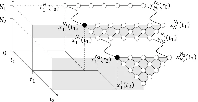
We illustrate the determinantal structure in Figure 3.
Proof of Theorem 4.1.Since the evolution is Markovian, we have
P(xN the lower index of all variables xkl is identically equal to 1.
The continuation of the proof requires a series of Lemmas collected at the end of this section, see Section 4.1. We apply Proposition 2.1 to them+1 factors in (4.28) (including the indicator function, which corresponds to the valuet=0 in Proposition 2.1). Namely,
0
Figure 3: A graphical representation of variables entering in the determinantal structure, illustrated form=2. The wavy lines represents the time evolution between t0 andt1 and from t1 tot2. The rest is the interlacing structure on the variables induced by the det[φn(· · ·)]. The black dots are the only variables which are not in the summation set D= D(0)∪D∗(t1)∪ · · · ∪D∗(tm) (see Figure 4 too). The variables of the border of the interlacing structures are explicitly indicated.
where we introduced the notationai:=a(ti)−a(ti−1), and bi:=b(ti)−b(ti−1).
First we collect all the factors coming from theQNi
n=1v
Thus, the probability we want to compute in (4.28) is obtained by a marginal of a measure onm+1 interlacing triangles, when we sum over all the variables in D(0),D∗(t1), . . . ,D∗(tm), see Figure 4
do the sum over the variables inD(tb i). Notice that the remaining variables in (4.30) do not belong
with the sum is over the variables described just above. By summing over thebD(ti), the determinant with FN include the terms in (4.30) into the ϕn’s by modifying the last row, i.e., by setting it equal to v
y
The identification to the expressions in Theorem 4.1 uses the representations (2.3) and (3.4).
The first line represent the initial condition att0 =0, the term with Ψ
N1
N1−l in Theorem 4.1. These
N1 variables evolves until time t1 and this is represented by the first line (termTt1,t0). After that, there is a reduction of the number of variables fromN1 toN2 by the interlacing structure, which is followed by the time evolution fromt1 to t2. This is repeated m−1 times. Finally it ends with an interlacing structure. IfN1=N2, then the first interlacing structure is trivial (not present), while if for examplet2=t1, then the time evolution is just the identity.
This corresponds to having a sort of vicious walkers with increasing number of walkers when the transition is made by theφ’s, and with constant number of walkers if the transition is the temporal one made byT.
The measure in (4.24) is written with the outer product over time moments but it can be rewritten by taking the outer product over the index nin the variables xkn’s. Let us introduce the following notations. For any levelnthere is a numberc(n)∈ {0, . . . ,m+1}of products of termsT which are give the expression for the kernel. Then we particularize it in case of the PushASEP with particle dependent jump rates. For this purpose, we introduce a couple of notations. For any two time moments tn1
a1,t
n2
a2, we define the convolution over all the transitions between them by φ
(tan11,t
which is an immediate corollary of (4.25). In a more general case considered in Theorem 4.2 below, if (4.39) does not holds, thenTn is just the convolution of the transitions between tnc(n)and t0n by
We remind that the variablesxkk−1in Mk,l are fictitious, compare with (4.27).
Theorem 4.2. Assume that the matrix M is invertible. Then the normalizing constant in (4.36) is equal to(detM)−1, the normalized measure2 of the form (4.36) viewed as(N1+. . .+Nm)-point process is
determinantal, and the correlation kernel can be computed as follows
In the case when the matrix M is upper triangular, there is a simpler way to write the kernel. Set
Φn,tna
The correlation kernel can then be written as
K(tn1
Moreover, one has the identity
φ(tna11,t on the formalism of[8]. The only place where the argument changes substantially is the definition of the matrix L, see[4], formula (3.32). We need to construct the matrix Lin such a way that its suitable minors reproduce, up to a common constant, the weights (4.36) of the measure. Then our measure turns into aconditional L-ensemblein the terminology of[8].
The variables of interest live in the spaceY=X(1)∪ · · · ∪X(N1), withX(n)=X(n) the matrix Lwritten with the order given by the entries in the set of all variablesX=I∪Ybecomes
with the matrix blocks inLhave the following entries:
[Ψ(N1)]
x,j = Ψ N1
N1−j(x), x ∈X
(N1)
0 ,j∈I, (4.49)
[En]i,y = (
φn+1(xnn+1,y), i=n+1,y∈X
(n+1)
c(n+1),
0, i∈I\ {n+1},y∈Xc(n(n++11)), (4.50)
[W[n,n+1)]x,y = φn+1(x,y), x ∈X
(n)
0 ,y∈X
(n+1)
c(n+1), (4.51)
andTnis the matrix made of blocks
Tn=
Tn,1 0 0
0 ... 0 0 0 Tn,c(n)
, (4.52)
where
[Tn,a]x,y =Ttn
a,tna−1(x,y), x ∈X
(n)
a ,y ∈X
(n)
a−1. (4.53)
The rest of the proof is along the same lines as that of Lemma 3.4 in[4].
Although the argument gives a proof in the case when all variables xan(tnb) vary over finite sets, a simple limiting argument immediately extends the statement to any discrete sets, provided the series that definesMk,l are absolutely convergent, which is certainly true in our case.
A special case of Theorem 4.2 is Proposition 3.1 stated in Section 3, which we prove below.
Proof of Proposition 3.1.We first prove the statement in the case the jump rates are ordered, v1 > v2>. . . , and then use analytic continuation invj’s.
For v1 > v2 > . . . , the claim is a specialization of Theorem 4.2. The kernel depends only on the actual times and particle numbers, therefore we might drop the label ai of t
ni
ai. Equivalently, we
can use the notation(ni,ti) instead of tni
ai, to go back to the natural notations of the model. For
PushASEP we haveΨN1
N1−l(x) =FN1+1−l,1(x−yl, 0, 0)and
Ttj,ti(x,y) =F1,1(x−y,a(tj)−a(ti),b(tj)−b(ti)). (4.54)
First of all, we sum over the{xN1
k (0), 1≤k≤N1}variables, since we are not interested in the initial conditions (being fixed). When applied to theFk,l(x,a(ti),b(ti)), the time evolutionTtj,ti changes
it intoFk,l(x,a(tj),b(tj)),
X
y∈Z
Ttj,ti(x,y)Fk,l(y,a(ti),b(ti)) =Fk,l(x,a(tj),b(tj)). (4.55)
This implies that Theorem 4.2 still holds but with tN1
0 =t1 and
ΨN1
N1−l(x) =FN1+1−l,1(x−yl,a(t1),b(t1)). (4.56)
We have, see (4.69), that
Using (4.55) and (4.57) repeatedly one then gets
which can be rewritten as (3.4).
Next we show that the matrix M is upper triangular. Once again, (4.55) and (4.57) are applied several times, leading to
(Note that we need the assumption vk>max{vl}l>kin order for this sum to converge.) We divide
the sum over y in two regions, {y ≥ 0} and{y <0}. The sum over y ≥ 0 can be taken into the that case the new pole at 1/vkdoes not have to vanish. The diagonal term is easy to compute, since
the pole at 1/vkis simple. Computing its residue we obtain Mk,k=v
Next, we need to determine the spaceVnwhere the orthogonalization has to be made. We have
(φk∗φ
As all the functionsΨnk,t, see (3.4), can be estimated as
|Ψnk,t(x)| ≤const·q|x|, x∈Z, (4.64)
for any q > 0 and v1,v2, . . . varying in a compact set, the weights (4.36) can be majorated by a convergent series forv1,v2, . . . varying in a compact set. Further, the normalizing constant(detM)−1 is analytic as long asvj’s are nonzero, see (4.61). Thus, the correlation functions of our measure are analytic invj’s.
Set, fork=0, . . . ,n−1,
fk(x) =
1 2πi
I
dz z−x−1
(1−vn−kz)(1−vn−k+1z)· · ·(1−vnz)
, (4.65)
where the integration contour includes the polesvn−−1k, . . . ,vn−1. Note that fk(x)is a linear combina-tion ofvnx−k, . . . ,vnx. Denote byG= [Gk,l]k,l=0,...,n−1the Gram matrix
Gk,l=X x∈Z
fk(x)Ψnl,t(x). (4.66)
Then forv1>v2>. . . we have
Φnk,t(x) = n−1
X
l=0
[G−1]k,lfl(x). (4.67)
Since the matrix M is triangular, G is also triangular. Its diagonal elements are easy to compute:
Gk,k = ea(t)vk+b(t)/vkvyk+1
k . Hence, (4.67) gives a formula forΦ’s that is analytic in vj’s as long as
they stay away from zero. This implies that the corresponding expression for the correlation kernel (3.3) is also analytic in vj’s, and thus both sides of the determinantal formula for the correlation
functions can be analytically continued. Finally, it is not difficult to see that the functions (4.65) span the spaceVn given by (3.1), which implies the statement.
4.1
Some lemmas
In this subsection we state and prove the Lemmas used in the proof of Theorem 4.2.
Lemma 4.3. Let us define the function
ϕn(x,y) = ¨
vny−x, y ≥x,
0, y <x. (4.68)
Then the following recurrence relations holds
Fk,l+1(x,a,b) = (ϕN+1−l∗Fk,l)(x,a,b) (4.69)
and
Fk−1,l(x,a,b) = (ϕN+2−k∗Fk,l)(x,a,b). (4.70)
From (4.70) andϕn(x,y) =ϕn(0,y−x) =ϕn(−y,−x)it follows
Fk−1,l(−x,a,b) =X y∈Z
x11(ti) x22(ti)
xNi+1−1
Ni+1−1(ti)
xNi+1
Ni+1(ti)
xNi
Ni(ti)
xNi+1−1 1 (ti) xNi+1
1 (ti) xNi−1
1 (ti) xNi
1 (ti) x Ni
2 (ti)
D(ti)
D∗(ti)
e D(ti)
b
D(ti) Db∗(ti)
Figure 4: A graphical representation of the summation domains that occurs in the next lemmas and theorem. The bold lines passes through the border of the domains.
Proof of Lemma 4.3.We have
Fk,l(x,a,b) =
1 2πi
I
Γ0
dzzx−1ebzea/z(1−vNz)· · ·(1−vN+2−kz)
(1−vNz)· · ·(1−vN+2−lz). (4.72)
Then applyingPy≥xvNy−+x1−lzy =zx/(1−vN+1−lz)(for|z| ≪1), we get that in the denominator we
have an extra factor, which corresponds to increasinglby one. Similarly, applyingϕN+2−k, the extra
factor in the denominator cancels the last one in the numerator, thus this is equivalent to decreasing
kby one.
We define the following domains, which will occurs several times in the following. A graphical representation is in Figure 4. Let us denote the set of interlacing variables at timeti by
D(ti) ={xnk(ti), 1≤n≤Ni, 1≤k≤n|xkn+1(ti)<xkn(ti)≤ xkn++11(ti)}. (4.73)
Then let
e
D(ti) ={xkn(ti)∈D(ti)|k≥2}, D(tb i) ={xkn(ti)∈D(ti)|n≤Ni+1−1}, (4.74)
and
D∗(ti) =D(ti)\ {xNi
1 (ti)}, Db∗(ti) =D∗(ti)\bD(ti). (4.75)
Lemma 4.4. We have the identity
dethFk,l(xNi+1−l
1 (ti)−x Ni+1−k
1 (ti−1),a,b)
i
1≤k,l≤Ni
= const X
e D(ti)
YNi
n=2
detϕn(xnk−1(ti),xln(ti))
1≤k,l≤n
× det
h
FNi+1−l,1(x
Ni
k (ti)−x1l(ti−1),a,b)
i
1≤k,l≤Ni