Full Terms & Conditions of access and use can be found at
http://www.tandfonline.com/action/journalInformation?journalCode=ubes20
Download by: [Universitas Maritim Raja Ali Haji] Date: 12 January 2016, At: 23:56
Journal of Business & Economic Statistics
ISSN: 0735-0015 (Print) 1537-2707 (Online) Journal homepage: http://www.tandfonline.com/loi/ubes20
Evaluation and Combination of Conditional
Quantile Forecasts
Raffaella Giacomini & Ivana Komunjer
To cite this article: Raffaella Giacomini & Ivana Komunjer (2005) Evaluation and Combination
of Conditional Quantile Forecasts, Journal of Business & Economic Statistics, 23:4, 416-431, DOI: 10.1198/073500105000000018
To link to this article: http://dx.doi.org/10.1198/073500105000000018
Published online: 01 Jan 2012.
Submit your article to this journal
Article views: 149
View related articles
Evaluation and Combination of Conditional
Quantile Forecasts
Raffaella G
IACOMINIDepartment of Economics, University of California, Los Angeles, P.O. Box 951477, Los Angeles, CA 90095-1477 (giacomin@econ.ucla.edu)
Ivana K
OMUNJERDivision of the Humanities and Social Sciences, California Institute of Technology, MC 228-77, Pasadena, CA 91125 (komunjer@hss.caltech.edu)
We propose an encompassing test for comparing conditional quantile forecasts in an out-of-sample frame-work. Our test provides a basis for forecast combination when encompassing is rejected. Its central features are (1) use of the “tick” loss function, (2) a conditional approach to out-of-sample evaluation, and (3) derivation in an environment with asymptotically nonvanishing estimation uncertainty. Our approach is valid under general conditions; the forecasts can be based on nested or nonnested models and can be obtained by general estimation procedures. We illustrate the test properties in a Monte Carlo experiment and apply it to evaluate and compare four popular value-at-risk models.
KEY WORDS: Encompassing; Generalized method of moments; Tick loss function; Value-at-risk.
1. INTRODUCTION
The vast majority of the economic forecasting literature has traditionally focused on producing and evaluating point fore-casts for the conditional mean of some variable of interest. More recently, increasing attention has been devoted to other characteristics of the unknown forecast distribution, besides its conditional mean, such as a particular conditional quantile.
A primary example of the growing interest in conditional quantile forecasts is in the context of risk management, as wit-nessed by the literature on value-at-risk (VaR) (e.g., Duffie and Pan 1997). Ever since August 1996, when U.S. bank regulators adopted a “market risk” supplement to the Basle Accord (1988), the regulatory capital requirements of commercial banks with trading activities are based on VaR estimates. This important measure of market risk is defined as the opposite of a pspecified quantile of the conditional distribution of portfolio re-turns, and its estimates are routinely generated by the banks’ internal models. There are a variety of approaches to esti-mating conditional quantiles in general and VaR in particular, ranging from parametric (e.g., Danielsson and de Vries 1997; Barone-Adesi, Bourgoin, and Giannopoulos 1998; Diebold, Schuermann, and Stroughair 1998; Embrechts, Resnick, and Samorodnitsky 1999; McNeil and Frey 2000), to semiparamet-ric (e.g., Koenker and Zhao 1996; Taylor 1999; Chernozhukov and Umanstev 2001; Christoffersen, Hahn, and Inoue 2001; Engle and Manganelli 2004; Komunjer 2005), to nonparametric (e.g., Battacharya and Gangopadhyay 1990; White 1992).
Given the range of techniques available for producing con-ditional quantile forecasts, it is necessary to develop adequate tools for their evaluation. A number of authors have focused on absoluteevaluation, that is, on testing whether a forecast-ing model is correctly specified or whether a sequence of forecasts satisfies certain optimality properties. For example, Zheng (1998) and Bierens and Ginther (2001) proposed spec-ification tests for evaluating a model against a generic alter-native. Christoffersen (1998) proposed a “correct conditional coverage” criterion for evaluating a sequence of interval fore-casts that does not require knowledge of the underlying model.
Corradi and Swanson (2002) allowed for misspecification and proposed a test that compares a reference model against generic nonlinear alternatives. A potential problem with absolute eval-uation is that if different models are rejected as being misspec-ified or if they are all accepted, then we are left without any guidance as to which one to choose. The approach of Corradi and Swanson (2002) is similarly inconclusive if the reference model is rejected. In this article, we thus focus onrelative eval-uation, which involves comparing the performance of compet-ing, possibly misspecified models or sequences of forecasts for a variable and choosing the one that performs the best. This approach was taken by Christoffersen et al. (2001), who pro-posed a method for comparing nonnested VaR estimates. These authors assumed that the VaR is a linear function of the volatil-ity and proposed estimating the parameters by the informa-tion theoretic alternative to generalized method of moments (GMM) due to Kitamura and Stutzer (1997). The evaluation of Christoffersen et al. (2001) was conducted in-sample and is valid only if the returns belong to a location-scale family (which implies that the VaR is a linear function of the volatility). Fur-ther, to apply their test, all VaR forecasts must be obtained by the estimation method of Kitamura and Stutzer (1997).
It is frequently the case, however, that good in-sample perfor-mance does not imply good out-of-sample perforperfor-mance and that the models underlying the forecasts remain partially or com-pletely unknown to the forecast user. Moreover, given the va-riety of approaches to estimating conditional quantile models outlined earlier, it may be of interest to investigate whether dif-ferent estimation techniques have an effect on forecast perfor-mance. In general, when several forecasts of the same variable are available, it is desirable to have formal testing procedures for out-of-sample comparison that do not necessarily require knowledge of the underlying model or, if the model is known,
© 2005 American Statistical Association Journal of Business & Economic Statistics October 2005, Vol. 23, No. 4 DOI 10.1198/073500105000000018
416
do not restrict attention to a specific estimation procedure. The goal of this article is to provide such a test.
Given an appropriate choice of loss function, one could in principle compare the out-of-sample average loss implied by alternative quantile forecasts using the tests of equal predictive ability proposed by Diebold and Mariano (1995), West (1996), White (2000), and Corradi and Swanson (2004). But these ap-proaches may not be applicable in several important cases, such as when the forecasts are from nested models or when they de-pend on semiparametric or nonparametric estimators.
In this article we choose a different approach and construct a test for out-of-sample conditional quantile forecast compari-son based on the principle of encompassing (e.g., Hendry and Richard 1982; Mizon and Richard 1986).
The novel features of our implementation of the principle of encompassing are first, the choice of the relevant loss function, which we argue to be the “tick” loss function; second, the fo-cus onconditionalexpected loss rather than unconditional ex-pected loss in the formulation of the encompassing test; and third, the derivation of our test in an environment with asymp-totically nonvanishing estimation uncertainty. These last two features link the approach in this article to that of Giacomini and White (2003), who proposed a general framework for out-of-sample predictive ability testing. Some of the advantages of this framework over that of, for instance, West (1996), are that it allows the forecasts to be generated by parametric models as well as by semiparametric or nonparametric techniques, and that it is applicable to both nested and nonnested forecast com-parisons. The implementation of our test makes use of standard GMM techniques. As a byproduct, our framework also provides a link to Christoffersen’s (1998) “correct conditional coverage” criterion for the absolute evaluation of interval forecasts.
A final feature of our encompassing approach is that it gives a theoretical basis for quantile forecast combination in cases when neither forecast encompasses its competitor. From a the-oretical viewpoint, forecast combination can be seen as a way to pool the information contained in the individual forecasts, and its benefits have been widely advocated since the early work of Bates and Granger (1969). According to Granger (1989), there are two situations when it is useful to combine forecasts. If the forecasts are based on the same information set, then a fore-cast combination can be useful only if the original forefore-casts are suboptimal according to the relevant loss function. But if the forecasts are instead based on different information sets, then combining them can potentially improve the forecasting per-formance by pooling the information contained in the two sets. Recent empirical work by Stock and Watson (1999, 2003) has further confirmed the accuracy gains induced by forecast com-bination for a large number of macroeconomic and financial time series. Surprisingly little empirical work has been done in the context of conditional quantile forecasting. Yet the benefits of expanding the information set through combination might be particularly evident for quantiles with small nominal coverage, as is usually the case for VaR. Extreme quantiles are very sensi-tive to the few observations in the tails of the empirical distrib-ution of the sample, and combining forecasts based on different information sets can thus be seen as a way to make the fore-cast performance more robust to the effects of sample-specific factors.
We illustrate the usefulness of the conditional quantile fore-cast encompassing (CQFE) test by applying it to the problem of VaR evaluation using S&P500 daily return data. We consider popular models for producing 1% and 5% VaR forecasts and generally conclude that the forecast combination outperforms the individual forecasts.
The remainder of the article is organized as follows. Sec-tion 2 describes the environment and gives an overview of our encompassing approach to comparing and combining compet-ing conditional quantile forecasts. Section 3 introduces the test for conditional quantile forecast encompassing and discusses the estimation problem underlying implementation of the test. A formal definition of the CQFE test statistic is provided in Theorem 1 in Section 3.2, which is the main result of this arti-cle. Section 4 analyzes the small-sample size and power prop-erties of the proposed test, and Section 5 applies the test to the problem of VaR forecast evaluation and combination. Section 6 concludes. The Appendix presents proofs. is a vector of explanatory variables. We are interested in the α-quantile of the distribution ofYt+1conditional on the
infor-mation setFt,Qt,α, defined as
Pt(Yt+1≤Qt,α)=α (1)
or
Qt,α≡F−t 1(α), (2) whereα∈(0,1),Ft is the conditional distribution function of Yt+1 andF−t 1 its inverse. Using the standard convention, the subscripttunder the probabilityP(·), distribution functionF(·), density f(·), expectation E[·]or α-quantile Qdenotes condi-tioning on the information setFt. To further simplify the nota-tion, we hereafter drop the reference to the indexαand simply denote the time t conditional α-quantile by Qt. As a general rule, a lower-case letter is used to denote observations of the corresponding random variable (e.g.,xtandXt).
Our goal is to propose a test for comparing alternative se-quences of one-step-ahead forecasts ofQt.We perform the eval-uation in an out-of-sample fashion. This involves dividing the sample of sizeTinto an in-sample part of sizemand an out-of-sample part of sizen, so thatT=m+n. The in-sample portion is used to produce the first set of forecasts, and the evaluation is performed over the remaining out-of-sample portion. We im-pose few restrictions on how the forecasts are produced. In par-ticular, they may be based on parametric models or be generated by semiparametric or nonparametric techniques. The forecasts can be produced using either a fixed forecasting scheme or a rolling window forecasting scheme. For example, for a para-metric model, a fixed forecasting scheme involves estimating the parameters only once on the firstmobservations and using
these estimates to produce all of the forecasts for the out-of-sample periodt=m+1, . . . ,T.A rolling window forecasting scheme, in contrast, implies reestimating the parameters at each out-of-sample point t using an estimation sample containing the mmost recent observations, that is, the observations from t−m+1 tot.
Let βˆt,m denote the k×1 vector collecting the time-t esti-mated parameters from the two models (for parametric forecast-ing) or whatever semiparametric or nonparametric estimator used in the construction of the forecasts. In what follows, we use the common notation βˆt,m for either forecasting scheme, with the understanding that a fixed forecasting scheme cor-responds to the case where βˆt,m = ˆβm,m for all t, m≤t ≤ T −1, whereas for the rolling window forecasting scheme,
ˆ
βt,m changes with t but depends only on the previousm ob-servations.
For simplicity, we restrict attention to pairwise comparisons, but all of the techniques can be readily applied to the case of multiple forecasts. For each time t, m≤t≤T−1, the one-step-ahead forecasts of Qt formulated at time t are denoted by qˆ1m,t≡q1(xt,xt−1, . . .; ˆβt,m) and qˆ2m,t≡q2(xt,xt−1, . . .;
ˆ
βt,m),whereq1andq2areFt-measurable functions.
The crucial requirement that we impose on the functions q1andq2 is that they are constant over time. This implies, in
particular, that use of an expanding estimation window (recur-sive forecasting scheme) is not allowed, whereas forecasting schemes using either a fixed or a rolling window of constant length satisfy the requirement. In the remainder of the article, we assume that the in-sample sizemis a finite constant, chosen by the user a priori. As a consequence, all of our results should be interpreted as being conditional on the given choice of m, but for ease of notation we choose not to make this dependence explicit (except forqˆ1m,tandqˆ2m,t).
2.2 Principles of Forecast Encompassing
Our approach to comparing conditional quantile forecasts is based on the principle of encompassing. Following, for exam-ple, Hendry and Richard (1982), Mizon and Richard (1986), and Diebold (1989), encompassing arises when one of two competing forecasts is able to explain the predictive ability of its rival. According to Clements and Hendry (1998, p. 228), a test for forecast encompassing can be generally defined as follows:
A test for forecast encompassing is a test of the conditional efficiency of a forecast, where a forecast is said to be conditionally efficient if the expected loss of a combination of that forecast and a rival forecast is not significantly less than the expected loss of the original forecast alone.
The two key ingredients of any forecast encompassing test are, therefore (1) the loss function involved in the computation of the expected loss and (2) the weights of the forecast combina-tion. The choice of the loss function is closely related to which characteristic of the unknown future distribution of the variable one wants to forecast. Letfˆt be a forecast of some characteris-tic of interest of the random variableYt+1,conditional on the
information set at time t.The forecast ˆft is said to be optimal at timetif it minimizesEt[L(Yt+1− ˆft)], whereLis some loss
function,L:R→R+. Note that the optimal forecast minimizes the expected lossconditionalonFt.As discussed in detail later,
the focus on conditional (rather than unconditional) expected loss is a central feature of our treatment of both evaluation and combination of forecasts and distinguishes our approach from related literature (e.g., Granger 1989; Taylor and Bunn 1998; Elliott and Timmermann 2004).
Different loss functions L correspond to different optimal forecasts. For example, lettinget+1≡yt+1− ˆft, if a quadratic loss functionL(et+1)=e2t+1is used, then the optimal forecast is
the conditional mean of the distribution ofYt+1. If, on the other
hand, an absolute value loss functionL(et+1)= |et+1|is used,
then the optimal forecast corresponds to the conditional median of the distribution ofYt+1. In this article the object of interest
isQt, the conditionalα-quantile of the distribution ofYt+1. The
corresponding loss function, L, is the asymmetric linear loss function of orderα,Tα, defined as
Tα(et+1)≡
α−1(et+1<0)et+1, (3)
which is also known as the “tick” or “check” loss function in the literature. We can thus argue that the tick functionT is the im-plicit loss function whenever the object of interest is a forecast of a particular quantile of the conditional distribution ofYt+1.
Regarding the choice of weights in the combination, in this article we restrict attention to linear combinations,(θ1t×
ˆ
q1m,t+θ2tqˆ2m,t),where(θ1t, θ2t)lies in some compact subset
ofR2. The values ofθ1tandθ2tcan be further constrained to lie in(0,1), withθ1t+θ2t=1,but we choose not to impose this restriction herein. (For a discussion of restrictions on the com-bination weights, see, e.g., Granger and Ramanathan 1984.) In the next section we formalize the concept of encompassing for conditional quantile forecasts.
2.3 Encompassing for Conditional Quantiles
Based on the general idea of Clements and Hendry (1998), we say that forecastqˆ1m,t encompasses forecastqˆ2m,t at timet if and only if
Et[Tα(Yt+1− ˆq1m,t)] ≤Et[Tα(Yt+1−(θ1tqˆ1m,t+θ2tqˆ2m,t)]
a.s.-P, for all(θ1t, θ2t)∈, (4) where is a compact subset of R2. In practice, testing the inequality (4) is not feasible, because it involves computing the expected loss for all (θ1t, θ2t)∈. Instead, let (θ1∗t, θ2∗t) denote the optimal set of weights, defined as a solution to the minimization problem min(θ1,θ2)∈Et[Tα(Yt+1 −(θ1 ×
Definition 1 (Conditional quantile forecast encompassing). Letqˆ1m,t andqˆ2m,tbe alternative forecasts forQt.qˆ1m,tis said
whereTα is the tick loss function defined in(3)and(θ1∗t, θ2∗t)is
The equivalence between (5) and (6) follows from the fact that the right side of (5) is the minimum of the conditional ex-pected loss over.
Comments.
1. If we interpret a conditional expectation as a prediction, then equality (5) can be viewed as saying that qˆ1m,t encom-passes qˆ2m,t if the forecaster cannot predict whether the op-timal combination of the two forecasts will outperform the original forecast at timet+1, given what is known at timet. This focus on prediction of future performance (conditional ex-pectation) rather than on assessment of average performance (unconditional expectation) in the definition of encompassing distinguishes our approach from the classic encompassing liter-ature (e.g., Hendry and Richard 1982; Mizon and Richard 1986) and establishes a link with the general framework for predictive ability testing proposed by Giacomini and White (2003).
2. Similar to Giacomini and White (2003), the forecasts
ˆ
q1m,tandqˆ2m,tin our definition of encompassing depend on the parameter estimates at timet, rather than on population values as in, for example, the approach of West (2001). This corre-sponds to a shift from evaluating a forecast model to evaluating the “forecast method,” which includes the model as well as the estimation procedure and the choice of estimation window.
3. Focusing on the actual forecasts rather than the underly-ing models in the definition of encompassunderly-ing means that we do not assume that the forecasts are estimated using the same tick loss function used for the evaluation. As a result, we provide a unified framework for comparing forecasts obtained by possi-bly different estimation techniques.
In the next section we discuss implementation of the CQFE test.
3. CONDITIONAL QUANTILE FORECAST ENCOMPASSING TEST
In what follows, we are interested in testing whetherqˆ1m,t conditionally encompassesqˆ2m,t over the entire out-of-sample period t=m, . . . ,T −1. Hereafter, we let θ≡(θ1, θ2)′ and
ˆ
qm,t≡(qˆ1m,t,qˆ2m,t)′. The following lemma expresses the op-timal weights in terms of the optimization problem’s first-order condition.
Lemma 1(Correct conditional coverage criterion). The vec-tor of optimal weightsθ∗t defined in (7) satisfies the following first-order condition:
Et[α−1(Yt+1−θ∗′t qˆm,t<0)] =0, a.s.-P. (8) It is interesting to note that (8) corresponds exactly to Christoffersen’s (1998) “correct conditional coverage criterion” for evaluating interval forecasts, here applied to the combina-tion forecastθ∗′t qˆm,t. What Lemma 1 shows is that the correct
conditional coverage condition is equivalent to requiring opti-mality of an interval forecast with respect to the tick loss func-tion.
We now discuss estimation of the optimal combination weights.
3.1 Generalized Method-of-Moments Estimation of Optimal Combination Weights
According to Definition 1,qˆ1m,t conditionally encompasses
ˆ
q2m,tfor allt,m≤t≤T−1 if and only ifθ∗m= · · · =θ∗T−1=
(1,0)′. In other words, the optimal combination weights are constant in time and equal to (1,0)′. By Lemma 1, it should therefore be the case that for e1=(1,0)′, E[(α−1(Yt+1−
e′1qˆm,t<0))Wt] =0, for allFt-measurable functionsWt and for all t, m≤t≤T−1. Let W∗t be anh×1 vector of vari-ables that are observed at time t and that contain all of the relevant information fromFt. We refer toW∗t as the “informa-tion vector.” As stated in Proposi“informa-tion 1, the general requirement on{W∗t}is that it is a strictly stationary and mixing series. As such, we allowW∗t to include previous forecasts (or measures of past forecast performance), provided that they are produced by either a fixed or a rolling window forecasting scheme. The reason for this is that in these two cases the forecasts are con-stant measurable functions of a finite window of data and thus inherit the properties of stationarity and mixing from the under-lying series. In practice, the choice ofW∗t depends on the na-ture of the application considered, as we discuss in more detail in Section 5. Further, denote byganh-vector-valued function
g:×R×Rh→Rhsuch that
g(θ;yt+1,w∗t)≡ [α−1(yt+1−θ′qˆm,t<0)]w∗t. (9) The key element in our implementation of the encompass-ing test is that under the null of encompassencompass-ing, we have E[g(e1;Yt+1,W∗t)] =0,and hence we can use Hansen’s (1982) GMM approach to estimate the solutionθ∗to the moment con-dition
g0(θ∗)≡E[g(θ∗;Yt+1,W∗t)] =0, (10) and then test whetherθ∗=e1. Given the out-of-sample portion
of size n=T−m, consisting of the sequence of observations (w∗′m,ym+1, . . . ,wT∗′−1,yT)′, the GMM estimator ofθ∗, denoted byθˆn, is defined as a solution to the minimization problem
min Using the fact that the first-order condition (8) implies that
{g(θ∗;Yt+1,W∗t),Ft} is a martingale difference sequence, a consistent estimator ofSis given by
ˆ
where θ˜n is some initial consistent estimate of θ∗. In cases when the information vector fails to incorporate all of the rel-evant information, condition g0(θ∗)=0 is no longer
equiva-lent to the first-order condition (8) and{g(θ∗;Yt+1,W∗t)}is no longer a martingale difference sequence. However,S can still be consistently estimated using some heteroscedasticity- and autocorrelation-robust estimator, like Newey and West’s (1987) estimator. We now focus on the asymptotic properties of the GMM estimatorθˆn.
Proposition 1 (Consistency). Assume that for everyt,m≤ t≤T−1, (a) the conditional density ofYt+1,ft(·), is contin-Assumption (b) is a mild condition ruling out the possibil-ity that the two sequences of forecasts are perfectly correlated, which would happen if, for example, the two models were pro-portional or differed only by a constant. One could in principle relax the assumption of strict stationarity in (c) and rely on ex-isting results on the consistency and asymptotic normality of GMM estimators for mixing sequences. However, we decided not to pursue this option, because it would cause the optimal weights to depend on the sample size, and thus result in a less intuitive formulation of the null hypothesis of encompassing. Conditions (d) and (e) are fairly standard and imply in particu-lar that all of the components of the information vector are not linearly dependent.
We now turn to the asymptotic distribution ofθˆn. The stan-dard asymptotic normality results for GMM require thatgn(θ) be once differentiable, which is not the case here. There are, however, asymptotic normality results for nonsmooth moment functions, hereinafter we use the one proposed by Newey and McFadden (1994). The basic insight of their approach is that a smoothness condition ongn(θ)can be replaced by the smooth-ness of its limitg0(θ), with the requirement that certain
remain-der terms are small. The asymptotic distribution ofθˆnis derived in the next proposition.
Proposition 2(Asymptotic normality). Let the assumptions of Proposition 1 hold and further assume that (f )E ˆqm,t4<∞;
Note that the expression forγn, which depends on the value of the conditional densityft evaluated at the optimal combina-tion of quantiles, is similar to the one commonly found in the quantile regression literature (e.g., Koenker and Bassett 1978; Komunjer 2005). Further, note that assumption (f ) implicitly places conditions on the existence of the finite-sample moments of the estimator on whichqˆm,tis based. encompasses qˆ1m,t. We propose a Wald test of hypotheses H10andH20in the following theorem.
Theorem 1(CQFE test). Let the assumptions of Proposition 2 hold. Consider the test statistics
Similar to the approach of Giacomini and White (2003), and in contrast to the existing predictive ability testing literature (e.g., West 1996; McCracken 2000), our asymptotic framework lets the number of out-of-sample observations go to infinity, while the in-sample size m remains finite. We adopt this as-sumption as a convenient way to obtain an environment with nonvanishing estimation uncertainty, which results in our test having several advantages. It can directly capture the effect of estimation uncertainty on forecast performance, it allows for general estimation procedure, and it can avoid the problems as-sociated with comparison of predictive ability involving nested models. To see why this is the case, suppose that we were com-paring nested models and that the smaller model were correctly specified. Letting the size of the estimation window go to in-finity would cause the parameter estimates to converge to their probability limits, which would render the forecasts from the two models asymptotically perfectly correlated, thereby invali-dating assumption (b) of Proposition 1.
Note that the assumption thatmis finite rules out using an ex-panding estimation window forecasting scheme. As noted by a referee, a drawback of requiring that observations from the dis-tant past be dropped from the estimation sample is that this may result in suboptimal parameter estimates in a stationary environ-ment. In principle, one could create an environment with non-vanishing estimation uncertainty in the context of an expanding estimation window forecasting scheme by assuming that the in-sample size grows more slowly than the out-of-in-sample size, but we decided against imposing this artificial condition here.
3.3 Test Implementation and Forecast Selection Implications
In the computation of the test statisticsENC1nandENC2n, defined in Theorem 1, we need a consistent estimator of the as-ymptotic covariance matrix=(γ′S−1γ)−1derived in Propo-sition 2. We estimate S using the sample variance of our moment vectorg,Sˆn≡ ˆS(θˆn), which is a fairly commonly used
estimator. The computation ofθˆn andSˆnis typically done re-cursively. We first choose anr×ridentity-weighting matrix,
Ir×r, in(11)and compute the correspondingθˆn,1. The resulting
new weighting matrix,Sˆ−n1(θˆn,1), is more efficient than the
pre-vious one, and solving (11) leads to a new estimatorθˆn,2. The
last two steps can then be repeated untilθnˆ,jequals its previous value,θˆn,j−1. UnlikeSˆn, our estimator of the matrixγ in (14) has a novel form, not yet seen in the literature. We let
ˆ derivative of a smooth approximation gn,τ(θ) to the sample
moment function gn(θ), defined as gn,τ(θ)≡n−1Tt=−m1{α−
[1−exp((yt+1−θ′qˆm,t)/τ )]1(yt+1−θ′qˆm,t<0)}w∗t (see, e.g., Bracewell 2000, pp. 63–65). Asτ goes to 0, the term inside the curly brackets converges toα−1(yt+1−θ′qˆm,t<0)and is hence a smooth approximation to the indicator function. The convergence ofγˆn,τ to its expected value is uniform inτ in a neighborhood of 0, which ensures that limτ→0γˆn,τ
p
→γ, as we show in the following lemma.
Lemma 2. Under the assumptions of Proposition 2, limτ→0γˆn,τ
p
→γ andˆn≡limτ→0(γˆn,τSˆ−n1γˆn,τ)−1
p
→. The CQFE test can then be implemented as follows. For a de-sired level of confidence, one first chooses the corresponding critical value cfrom the χ22 distribution. If ENC1n≤c, then we conclude thatqˆ1m,t encompassesqˆ2m,t. IfENC2n≤c,then we infer thatqˆ2m,t encompassesqˆ1m,t. If instead bothENC1n andENC2nc, then the final conclusion is thatqˆ1m,tdoes not encompassqˆ2m,tandqˆ2m,tdoes not encompassqˆ1m,t. The con-ditional encompassing test for quantile forecasts can be easily generalized to the comparison ofr forecasts (or, more gener-ally,rweights). In this case, the limiting distribution of the test statistic will beχr2.
One important application of our CQFE test is in the con-text of real-time forecast selection, that is, for selecting at time T a best forecast method for timeT+1.To this end, we pro-pose the following decision rule. Perform the two tests ofH10
(qˆ1m,t encompassesqˆ2m,t)andH20 (qˆ2m,t encompasses qˆ1m,t)
on data up to timeT.There are four possible scenarios: (1) If neitherH10 nor H20 are rejected, then the test is not helpful
for forecast selection (one could, e.g., decide to use the more parsimonious model); (2) ifH10is rejected whileH20is not
re-jected, then one would chooseqˆ2m,T;(3) ifH20is rejected while H10 is not rejected, then one would choose qˆ1m,T;(4) if both H10andH20are rejected, then one would choose the
combina-tion forecastqˆcm,T≡ ˆθ1nqˆ1m,T+ ˆθ2nqˆ2m,T,whereθˆ1nandθˆ2nare out-of-sample estimates of the combination weights.
4. MONTE CARLO EVIDENCE
We investigate the performance of our CQFE test in finite samples of sizes typically available to financial economists. We perform the evaluation along three dimensions: the size of the
test, its power, and its sensitivity to the choice ofτ in the con-struction of γˆn,τ in (17). We design our Monte Carlo experi-ment to match the problem of VaR evaluation and combination that is the object of our empirical application. For simplicity, we restrict attention to the conditional autoregressive value at risk (CAViaR) family of VaR models proposed by Engle and Manganelli (2004). Our choices of models within the CAViaR family and the parameter values used for the simulation are driven by the empirical application.
4.1 Size Properties
We consider forecasts generated by the asymmetric absolute value (AAV) CAViaR model,
VaRAAV,t+1=β0+β1VaRAAV,t+β2|rt−β3|, (18)
and by the symmetric absolute value (SAV) model,
VaRSAV,t+1= ˜β0+ ˜β1VaRSAV,t+ ˜β2|rt|, (19) whereVaRAAV,t+1 andVaRSAV,t+1 are forecasts of the
condi-tionalα-quantile of−rt+1. Our null hypothesis is that the AAV
model encompasses the SAV model. To generate data that sup-port the null hypothesis, we proceed as follows. First, we fix the values of the true parameters(β0, β1, β2, β3)and(β˜0,β˜1,β˜2)
in (18) and (19), and replicate (VaRAAV,1, . . . ,VaRAAV,n)and
(VaRSAV,1, . . . ,VaRSAV,n) by assuming that rt∼iidN(0, σ2) withσ =.1. In this particular case, the in-sample sizemis 0 andT=n. Accordingly, all inference is done conditional on the set of true parameter values (β0, β1, β2, β3)and(β˜0,β˜1,β˜2).
Next, we constrainVaRAAV,t+1to be the conditionalα-quantile
of −rt+1 by redefining the original series. For every t, t=
0, . . . ,n−1, we let the data-generating process (DGP) be rt+1= −VaRAAV,t+1+ut+1, (20)
withut+1∼iidN(−σ −1(α), σ2),σ=.1, whereis the
dis-tribution function of a standard normal random variable. By re-stricting ut+1 to have theα-quantile of 0, we ensure that the
AAV model in (18) produces forecasts of the true conditional α-quantile of−rt+1.
The parameter values(β0, β1, β2, β3)=(0, .8, .3,1)in (18)
and(β˜0,β˜1,β˜2)=(0, .9, .2)in (19) are chosen so as to match
the estimates obtained in the empirical application forα=5%. We consider a range of values for the out-of-sample size n and the parameter τ in (17):n=(1,000,2,500,5,000)and τ ranges from.2×10−2to 10−2in increments of .1×10−2. For each sample size n, we generate 30,000 Monte Carlo replications of the time series {rt}nt=1, {VaRAAV,t}nt=1, and
{VaRSAV,t}nt=1, each of length n. We then consider the fore-cast combination (θ0+θAAV ·VaRAAV,t +θSAV·VaRSAV,t) and construct the GMM estimator (θˆ0n,θˆAAVn,θˆSAVn)′ of the
optimal weight vector (θ0∗, θAAV∗ , θSAV∗ )′ according to the pro-cedure described in Section 3. Note that we include a con-stant term in the forecast combination, thus allowing the empirical coverage of the original forecasts to be different than the 5% nominal value. In our particular case, the AAV forecasts will display correct empirical coverage by construc-tion, whereas the forecasts from the misspecified SAV model will in general be biased. Finally, we compute the proportion of rejections, at the 5% nominal level, of the null hypothesis
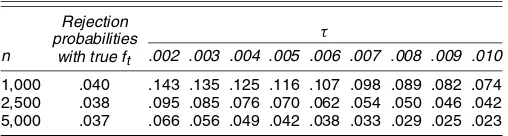
Table 1. Empirical Size of Nominal .05 Test
Rejection probabilities
with true ft
τ
n .002 .003 .004 .005 .006 .007 .008 .009 .010
1,000 .040 .143 .135 .125 .116 .107 .098 .089 .082 .074 2,500 .038 .095 .085 .076 .070 .062 .054 .050 .046 .042 5,000 .037 .066 .056 .049 .042 .038 .033 .029 .025 .023
NOTE: Empirical size of the CQFE test for a nominal size of .05. Rejection frequencies are computed over 30,000 Monte Carlo replications of the null hypothesis that forecasts from the AAV CAViaR model encompass forecasts from the SAV CAViaR model when the DGP is the AAV CAViaR.nis the sample size, andτis a user-defined constant required in the computation of our estimator ofγin (17).
H10:(θAAV∗ , θSAV∗ )=(1,0). The test statisticENC1nis that of Theorem 1, with ˆ substituted byRˆR′, so as to reflect the appropriate parameter restrictions. The information vectorW∗t
is W∗t ≡(1,rt,VaRAAV,t,VaRSAV,t)′. The results are collected in Table 1.
The nominal 5% test appears to be well sized, with rejection probabilities around 4% across all sample sizesn, when we es-timate γ in (14) using the true conditional density ft of rt+1
in (20). In a more plausible setup in which the true densityftis unknown and where we estimateγ by using our estimatorγˆn,τ
in (17), the empirical rejection probabilities vary with the sam-ple sizenand the smoothing parameterτ. A general pattern that emerges from Table 1 is that the test is oversized forn=1,000 and small values ofτ (.2×10−2) and is moderately undersized forn=5,000 and large values ofτ (10−2). For other combina-tions ofnandτ, the test appears generally well sized.
4.2 Power Properties
To generate data under the alternative hypothesis of no en-compassing of AAV forecasts with respect to SAV forecasts, we
first replicate (VaRAAV,1, . . . ,VaRAAV,n) and (VaRSAV,1, . . . , VaRSAV,n)for parameter values(β0, β1, β2, β3)=(0, .8, .3,1)
and(β˜0,β˜1,β˜2)=(0, .9, .2), following the procedure described
in the previous section, and then let the DGP be
rt+1= −[ρVaRSAV,t+1+(1−ρ)VaRAAV,t+1] +ut+1, (21)
where 0< ρ <1 and ut+1∼iidN(−σ −1(α), σ2), σ =.1,
as in the previous section. Note that the size study is obtained when the data are generated according to (21) withρ=0. Ac-cordingly, increasingρtoward 1 allows us to obtain the power curve for the CQFE test. We consider a number of different values for ρ, ranging fromρ =.02 to ρ =1, in increments of.02. For each parameterization, we generate 30,000 Monte Carlo replications of the time series{rt}nt=1,{VaRAAV,t}nt=1, and
{VaRSAV,t}nt=1and proceed as previously by computing the pro-portion of rejections of the null hypothesis thatVaRAAV,t+1
en-compasses VaRSAV,t+1 at the 5% nominal level. Figure 1(a)
plots the power curves forn=(1,000,2,500,5,000)when us-ing the true conditional densityftin the expression (14) forγ. As expected, the power increases withn. The loss of power in-duced by estimatingγwith our estimatorγˆn,τ in (17) is shown in Figure 1(b) for the case wheren=2,500 and for different values of the smoothing parameterτ. This figure highlights the trade-off between size and power when choosing a particular value ofτ. For example, high values ofτ (10−2) give a well-sized test (4.2% empirical size) but with low power (40% of rejections ofH10 whenH20 is true), whereas low values of τ
(.2×10−2) result in better power (70% of rejections ofH10
whenH20 is true) at the expense of size distortions (9.5%
em-pirical size).
(a) (b)
Figure 1. Power Curves of the CQFE Test in the Monte Carlo Experiment Discussed in Section 4.2 for (a) Known Density and (b) n=2,500. Each curve represents the rejection frequency—computed by assuming ftin (14) known—over 30,000 Monte Carlo replications. The null hypothesis being
tested is that forecasts from the AAV CAViaR model encompass forecasts from the SAV CAViaR model when the DGP is a convex combination of the two, with weightsρand (1−ρ). [(a), n=1,000; n=2,500; n=5,000; (b) known density; estimated density withτ=.010; estimated density withτ=.006; estimated density withτ=.002.]
5. EMPIRICAL EVALUATION AND COMBINATION OF VALUE–AT–RISK FORECASTS
Here we illustrate the potential usefulness of our CQFE test by applying it to the problem of VaR evaluation. The impor-tance of VaR became institutional in August 1996, when U.S. bank regulators adopted a “market risk” supplement to the Basle Accord of 1988. VaR has thus become a risk measure for setting capital-adequacy standards of U.S. commercial banks. The data used in our empirical application consist of 16 years of daily returns on the S&P500 index (source: Datastream), from September 1985 to September 2001 (T=4,176 observa-tions). The first third of the sample, corresponding to the period from September 1985 to January 1991 (m=1,392 observa-tions) is used as the in-sample period, while the remaining two thirds (n=2,784 observations) are reserved to evaluate the out-of-sample performance. We adopt a fixed forecasting scheme, which means that all forecasts depend on the same set of pa-rameters estimated over the firstmobservations. We consider a portfolio consisting of a long position in the index, with an investment horizon of 1 day.
5.1 VaR Models
We consider the 5% and 1% VaR forecasts originated from four different models: VaR1,t+1 and VaR2,t+1 are VaR
fore-casts based on conditional heteroscedasticity models,rt+1|Ft∼ D(0, σt2+1)withDbelonging to a location-scale family of dis-tributions. In this case VaR is a linear function of the condi-tional volatility of the returnsσt+1, and different VaR models
correspond to different specifications for the conditional vari-ance σt2+1. Two such specifications are the commonly used GARCH(1,1)model, in whichσ12,t+1=ω0+ω1σ12,t+ω2r2t, and the J. P. Morgan (1996) RiskMetrics model, where the variance is obtained as an exponential filterσ22,t+1=λσ22,t+ (1−λ)r2t, withλ=.94 for daily data. In both cases the corre-sponding VaR model is
VaRi,t+1=β0+β1σi,t+1, i=1,2. (22)
Models such as (22) have been studied by Christoffersen et al. (2001), among others. Hereafter, we refer to VaR1,t+1 as
GARCH VaR and toVaR2,t+1as RiskMetrics VaR.
A different approach to VaR modeling and estimation was taken by Engle and Manganelli (2004). Here we consider two examples of the CAViaR model proposed by these authors. VaR3,t+1is a forecast based on an asymmetric absolute value
(AAV) model,
VaR3,t+1=β0+β1VaR3,t+β2|rt−β3|, (23)
whereasVaR4,t+1is based on an asymmetric slope (AS) model, VaR4,t+1=β0+β1VaR4,t+β2rt++β3rt−, (24) wherer+t andr−t correspond to the positive and negative parts of rt. The three models VaR1,t+1, VaR3,t+1, andVaR4,t+1 are
chosen on the basis of their individual performance in model-ing the VaR for the S&P500 index. As shown by Christoffersen et al. (2001), the GARCH VaRVaR1,t+1is the only VaR
mea-sure among several alternatives considered by the authors that passes the Christoffersen (1998) “conditional coverage test”
for both 5% and 1% coverage rates. Similarly, Engle and Manganelli (2004) showed that the AAV model VaR3,t+1and
the AS model VaR4,t+1 are the best CAViaR specifications
for the S&P500 according to a criterion that they proposed. Fi-nally, the J. P. Morgan (1996) RiskMetrics model VaR2,t+1 is
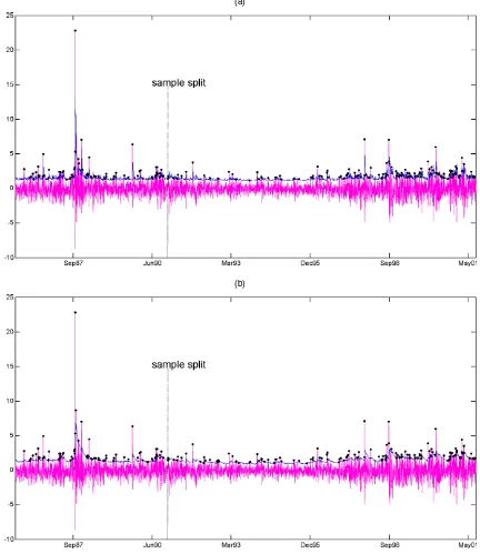
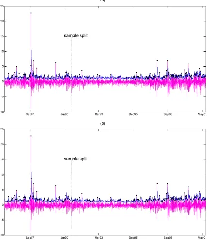
chosen as a benchmark model commonly used by practition-ers. Figures 2 and 3 show the out-of-sample sequences of VaR forecasts generated by the foregoing models, together with the sequences of VaR violations.
For each of the four VaR models (22)–(24), we first con-struct an estimator,βˆm≡ ˆβm,m, of the unknown parameter vec-torβ by using the first m=1,392 observations. We then use this estimator to form out-of-sample VaR forecasts according to a fixed forecasting scheme. In other words, at each out-of-sample datet,m≤t≤T −1, we compute one-step-ahead VaR forecasts, VaRi,t+1,i=1,2,3,4, based on the four
mod-els (22)–(24). The computation is done recursively, meaning that for each i=1,2,3,4, the value ofVaRi,t+1 depends on
the past forecastVaRi,t[σi2,tin the case of models (22)] and on the out-of-sample realization rt (resp.r2t). For illustration, we report the parameter estimatesβˆmin Table 2. Alternatively, one could consider sequences of VaR forecasts provided by differ-ent groups of outside researchers/analysts without knowing the underlying forecasting models, as long as the latter satisfy our assumptions.
As a quick check of the out-of-sample performance of in-dividual VaR models and their equally weighted pairwise combinations (.5·VaRi,t+1+.5·VaRj,t+1), we compute the
empirical coverage a, of the corresponding sequence of fore-casts, a≡n−1n
t=1It+1, where It+1 denotes the “hit”
vari-able It+1≡1(Yt+1−VaRt+1 <0). If the VaR model under
consideration performs well, then we expect it to display cor-rect unconditional coverage, attained when the empirical cov-erage a equals the nominal coverage α. Note that one could devise a simple likelihood ratio test of the null hypothesis that It+1 is Bernoulli(α), which is the main principle of the
so-called “unconditional coverage” test discussed by, among others, Christoffersen (1998). But this test assumes away para-meter estimation uncertainty, and thus we decided not to report its results here. The out-of-sample empirical coverages are re-ported in Table 3.
Based on the results from Table 3, we can compare VaR mod-els in terms of the difference between their out-of-sample em-pirical coverageaand the nominal coverageα. Forα=1%, the best model is GARCH(1,1)with empirical coverage .853%, followed by three equally performing models with coverage .742%: AAV and equally weighted combinations of GARCH with RiskMetrics and AS. Forα=5%, the best empirical cov-erage (4.970%) is that of RiskMetrics, followed by an equally weighted combination of RiskMetrics and GARCH (4.711%) and GARCH alone (4.674%). It is interesting to note that in general, the unconditional coverage of equally weighted combi-nations(.5·VaRi,t+1+.5·VaRj,t+1)is between that ofVaRi,t+1
andVaRj,t+1.
To assess the relative performance of the two models with the best empirical coverages, as identified earlier, we perform our CQFE test. Specifically, we test whether (1) atα=1% level, GARCH encompasses AAV, and (2) at α=5% level, Risk-Metrics encompasses GARCH. Note that before applying the
(a)
(b)
Figure 2. In- and Out-of-Sample Daily Series of Percentage Losses on S&P500 Index With 5% VaR From the (a) GARCH VaR and (b) RiskMet-rics Models. VaR violations (or hits) are represented by dots.
CQFE test, we must verify that the sequences of forecasts are not perfectly correlated. The out-of-sample correlation coeffi-cients are .91 for case (1) and .86 for case (2), which allows us to conclude that assumption (b) in Proposition 1 is not violated.
5.2 CQFE Test Results
We estimate the optimal combination weights (θ0∗, θi∗, θj∗)′ in the forecast combinationθ0+θiVaRi,t+θjVaRj,t using the GMM approach described in Section 3. For the purposes of this empirical application, we letW∗t ≡(1,rt,VaRi,t,VaRj,t)′.
We report the estimated combination weightsθˆ0n,θinˆ , andθjnˆ together with their standard errors, in Table 4. It is important to
note that the computation of standard errors is based on our es-timatorγˆn,τ given in (17), in which the smoothing parameterτ takes values.2×10−2,.6×10−2, and 10−2. For these values ofτ, the CQFE test has reasonable size and power properties, as shown in the Monte Carlo exercise. Table 4 also contains the corresponding values of the test statisticsENCinandENCjn.
As can be seen from Table 4, neither forecast encompasses its competitor for both levels ofα.This implies that the forecast combination in both cases outperforms the individual forecasts. However, note that forα=5%, the weight on the RiskMetrics forecast is not significantly different from 0 (t-statistics range from.046 to.074), suggesting that the optimal combination in this case is simply the bias-corrected GARCH forecast.
(a)
(b)
Figure 3. In- and Out-of-Sample Daily Series of Percentage Losses on S&P500 Index With 5% VaR From the (a) AAV and (b) AS Models. VaR violations (or hits) are represented by dots.
6. CONCLUSION
In this article we propose a CQFE test for comparing alter-native conditional quantile forecasts in an out-of-sample frame-work. We base our evaluation on the concept of encompassing, which requires that a forecast be able to explain the predictive ability of a rival forecast. The CQFE test thus can be viewed as a test of superior predictive ability. The setup proposed in this article also allows us to discuss the benefit of forecast combi-nation for quantile forecasts, which becomes relevant when the encompassing tests indicate that neither forecast outperforms its competitor.
The key features of our approach are (1) the use of the tick loss function rather than the quadratic loss function in the definition of encompassing; (2) a conditional, rather than un-conditional, approach to out-of-sample evaluation; and (3) the derivation of our test in an environment with asymptotically nonvanishing estimation uncertainty. Some of the benefits of our approach are that it allows comparison of forecasts based on both nested and nonnested models and of forecasts produced by general estimation procedures.
Implementation of the CQFE test is done using a fairly standard GMM estimation technique, with the optimization procedure appropriately modified to accommodate our
Table 2. VaR Parameter Estimates
ˆ
β0 βˆ1 βˆ2 βˆ3
α=.01
GARCH .982 1.597
(.048) (.033)
RiskMetrics .959 1.698
(.104) (.125)
AAV .213 .714 .761 .422
(.020) (.040) (.068) (.026)
AS .460 .716 .110 −.796
(.029) (.061) (.011) (.081)
α=.05
GARCH .055 1.446
(.075) (.095)
RiskMetrics .500 1.039
(.104) (.137)
AAV −.074 .804 .328 1.070
(.008) (.016) (.015) (.065)
AS .120 .834 .025 −.404
(.048) (.058) (.006) (.123)
NOTE: Parameter estimates for different VaR models. Data are Datastream daily returns on S&P500 from September 1985 to January 1991 (m=1,392 observations). The estima-tion is carried out by GMM in the GARCH and RiskMetrics VaR models and by QML in the CAViaR models. For VaR models wherert+1|Ft∼N(0,σt2+1) with (1) GARCH volatility σ2
t+1=ω0+ω1σt2+ω2rt2we haveω0=.117,ω1=.763, andω2=.150, and for those with (2) RiskMetrics volatilityσ2
t+1=λσt2+(1−λ)rt2we takeλ=.94.
ferentiable criterion function. The CQFE test displays good size and power properties for samples of sizes typically available in financial applications.
We apply the CQFE test to the problem of conditional VaR forecast evaluation using S&P500 daily index returns. At the 1% level, we find that a forecast combination (with intercept) of GARCH and AAV CAViaR forecasts outperforms both indi-vidual components. A similar result holds at 5% level, where we compare VaR forecasts generated from RiskMetrics and GARCH models. In the latter case, however, we find that the combination weight on the RiskMetrics forecast is not signifi-cantly different from 0, indicating that bias-corrected GARCH forecasts for the 5% VaR encompass RiskMetrics forecasts.
ACKNOWLEDGMENTS
The authors thank Graham Elliott, Clive Granger, Jose Lopez, Andrew Patton, and Kevin Sheppard, as well as the par-ticipants to the 2003 ASSA meeting in Washington, DC, UTS workshop, and Duke Conference on Forecasting, for their valu-able comments and suggestions, and Peter Christoffersen and
Table 3. Out-of-Sample Empirical Coverage
GARCH RiskMetrics AAV AS
α=.01
GARCH .853% .742% .705% .742%
RiskMetrics .705% .705% .631%
AAV .742% .668%
AS .631%
α=.05
GARCH 4.674% 4.711% 4.191% 4.191%
RiskMetrics 4.970% 4.228% 4.191%
AAV 4.303% 4.303%
AS 4.228%
NOTE: Empirical coveragea=n−1I
t+1for individual VaR models (diagonal elements) and
their equally weighted pairwise combinations (off-diagonal elements). Data: Datastream daily returns on S&P500 from January 1991 to September 2001 (n=2,784 observations).
Eric Ghysels for providing their data. They also thank the edi-tors, the associate editor, and two anonymous referees for their useful comments that led to a considerably improved version of the article. Any remaining errors are the authors’ own.
APPENDIX: PROOFS
We use the following notation throughout. If V is a real n-vector, V≡(V1, . . . ,Vn)′, then V denotes the L2-norm
of V, that is, V2≡V′V=n
i=1Vi2. If M is a real n×n -matrix, M≡(Mij)1≤i,j≤n, then M denotes the L∞-norm
ofM, that is,M ≡max1≤i,j≤n|Mij|. Proof of Lemma 1
Let
t(θ)≡Etα−1(Yt+1−θ′qˆm,t<0)(Yt+1−θ′qˆm,t)
=
R
α(yt+1−θ′qˆm,t)dFt(yt+1)
−
R1
(yt+1−θ′qˆm,t<0)(yt+1−θ′qˆm,t)dFt(yt+1)
=
+∞
−∞
α(yt+1−θ′qˆm,t)dFt(yt+1)
−
0
−∞
xt+1dFt(xt+1+θ′qˆm,t),
Table 4. Conditional Quantile Forecast Encompassing Test for VaR Measures
Model θˆ0n θˆ1n θˆ2n J ENC1n ENC2n
α=.01
GARCH(1) versus AAV(2) −1.506 1.048 .382 8.636
τ=.002 (.248) (.147) (.748) 70.779∗ 69.224∗
τ=.006 (.298) (.158) (.074) 53.104∗ 71.181∗
τ=.010 (.392) (.209) (.089) 40.071∗ 48.335∗
α=.05
RiskMetrics(1) versus GARCH(2) −.118 .005 .565 10.545
τ=.002 (.057) (.068) (.092) 602.510∗ 150.690∗
τ=.006 (.066) (.086) (.102) 260.544∗ 96.291∗
τ=.010 (.083) (.109) (.125) 152.563∗ 61.207∗
NOTE: Out-of-sample CQFE test for VaR measures for a portfolio composed of a long position in S&P500 index with an investment horizon of 1 day. Data are Datastream daily returns on S&P500 from January 1991 to September 2001 (n=2,784 observations). The consistent standard errors of the GMM estimator (θ0n,θ1n,θ2n)′were computed withτ=.002,.006,.010 and are reported in parentheses.Jis the value of theJ-test statistics:J=
gn(θn)′S−1gn(θn). The marked (∗) values of the CQFE test statisticsENC1nandENC2nare significant at the 1% level.
where xt+1 ≡ yt+1 − θ′qˆm,t. Thus ∇θt(θ) = −αqˆm,t − 0
−∞qˆm,txt+1ft(xt+1+θ′qˆm,t)dxt+1, because we assume that
the random variable Yt+1 has a continuously differentiable
conditional density ft, that is, dFt(yt+1)=ft(yt+1)dyt+1 and ft continuous. By arranging the previous equality, we ob-tain ∇θt(θ)= −αqˆm,t − [ˆqm,txt+1ft(xt+1 +θ′qˆm,t)]0−∞ + Because qˆm,t is Ft-measurable, we can rewrite the previous equation asEt[α−1(Yt+1−θ∗′t qˆm,t<0)] =0, a.s.-P, CQFD.
Proof of Lemma A.1. By contradiction, suppose there ex-ist (γ1, γ2)=(0,0) such that γ1qˆ1m,t +γ2qˆ2m,t =0, a.s.-P.
Lemma A.2. Under assumptions (a) and (b) of Proposition 1, θ∗is unique. becauseW∗t isFt-measurable. The conditional expectation on the right side of the equality is in turn equal toθ¯′qˆm,t
θ∗′qˆm,tft(yt+1) dyt+1≡Dt(θ¯,θ∗). Thus (Wt∗)=E[W∗tDt(θ¯,θ∗)], and we have(W∗t)=0⇒Dt(θ¯,θ∗)=0, a.s.-P, given that W∗t in-corporates all available information inFt. By assumption (a), ft(·)is continuous and strictly positive onR, so thatDt(θ¯,θ∗)
andqˆm,t.Consider the cases of fixed forecasting scheme and rolling window forecasting scheme separately.
For a fixed forecasting scheme, the forecasts qˆm,t, t =
m, . . . ,T−1, depend on the one hand on predetermined pa-rameter estimates βˆm,m, hence on the variables (X1, . . . ,Xm), and on the other hand on some set of right-side variables of the forecasting model that are observed at timet. Typically, those variables are included in the vector W∗t. Therefore, by letting
Vt+1≡(Yt+1,W∗t,X1, . . . ,Xm)′, we can rewriteg(θ;Yt+1,W∗t) asg(θ;Vt+1).
For a rolling window forecasting scheme, qˆm,t, t=m, . . . ,
T−1, is a constant measurable function of the estimation win-dow, which consists of themmost recent observations ofXt. In that case, we can again letVt+1≡(Yt+1,W∗t,Xt, . . . ,Xt−m+1)′
and rewriteg(θ;Yt+1,Wt∗)asg(θ;Vt+1).
Because for every t, t=m, . . . ,T−1,Vt+1 is a function
of a finite number (m+2) of variables which, by assump-tion (c), are strictly staassump-tionary and α-mixing, the sequence
{Vt} is strictly stationary and α-mixing of the same size (see, e.g., thm. 3.49 in White 2001). Note that strict sta-tionarity and α-mixing of {Vt} imply ergodicity (see, e.g., thm. 3.44 in White 2001), so that we can use one of the stan-dard results on the consistency of GMM estimators for sta-tionary and ergodic sequences. Specifically, we verify that the conditions of thm. 2.6 of Newey and McFadden (1994, pp. 2132–2133) are satisfied in our case. (Note that the re-sults of thm. 2.6 hold if the iid assumption is replaced with the condition that{Vt}is strictly stationary and ergodic.) First, we need to show that Sˆn(θˆn)→p S, where S is defined in (12) and, from (13),Sˆn(θ)≡n−1Tt=−m1g(θ;Vt+1)g(θ;Vt+1)′.
Note thatg is anFt+1-measurable function of{Vt+1}, which
is strictly stationary and α-mixing. Using, once again, theo-rem 3.49 of White (2001), we then have that{g(θ;Vt+1)}and
{g(θ;Vt+1)g(θ;Vt+1)′}are strictly stationary andα-mixing of
same size. Hence we can apply a law of large numbers (LLN) for α-mixing sequences to show that for every θ∈,Sˆn(θ) converges toS˜(θ)≡E[g(θ;Vt+1)g(θ;Vt+1)′]. Specifically, we
check that the assumptions of corollary 3.48 of White (2001) hold. First, note that for r>2, we have −r/(r−1) >−r/
Moreover, we know (by norm equivalence) that there exist some positive constantcsuch that
so by letting 2δ˜=δ and using assumption (e), we getEg(θ;
particular, ifθˆnis some previously obtained consistent estimate of θ∗, then Sˆn(θˆn)
p
→ ˜S(θ∗) = E[g(θ∗;Vt+1)g(θ∗;Vt+1)′],
which, due to the fact that {g(θ∗;Vt+1),Ft} is a martingale difference sequence, equals the asymptotic covariance matrixS
in (12).
We now check that all the other conditions of theorem 2.6 of Newey and McFadden (1994) are satisfied; in particular, we have S=E[g(θ∗;Yt+1,W∗t)g(θ∗;Yt+1,W∗t)′] = E{[α− equality implies thatζ needs to be equal to anh-vector of 0’s. Hence the matrices S and its inverse S−1 are positive def-inite. In particular, this implies that S−1E[g(θ;Vt+1)] =0
only if E[g(θ;Vt+1)] =0. This, together with Lemma A.2,
verifies condition 2.6(i). Condition 2.6(ii) is the standard compactness condition on the parameter space that we impose here. The continuity condition 2.6(iii) holds because
g(θ;Vt+1) is a.s. continuous on . Indeed, note that the
only discontinuity point occurs when Yt+1=θ∗′qˆm,t, a.s.-P, which, due to the continuity of Yt+1, occurs with
probabil-ity 0. Finally, condition 2.6(iv) is verified by imposing assump-tion (e), because for allθ∈, we haveg(θ;Vt+1) ≤ W∗t,
Lemma A.3. Let the assumptions of Proposition 1 hold. We then have√ngn(θˆn)
p
→0.
Proof of Lemma A.3. Recall from (11) that θˆn minimizes
[gn(θ)]′Sˆ−n1[gn(θ)] on , where gn(θ) = n−1T−1
where we have used the fact thatYt+1is a continuous random
variable, so thatn−1T−1
t=m1(Yt+1= ˆθ′nqˆm,t)Wt∗,j=op(1). Us-ing condition (A.2), finally the foregoUs-ing inequality implies that
√n
gn(θˆn) p
→0, CQFD. Proof of Proposition 2
We check that all the conditions of theorem 7.2 of Newey and McFadden (1994, p. 2186) are verified. We first need to check that gn(θˆn) verifies an “asymptotic first-order con-dition,”gn(θˆn)′Sˆn−1gn(θˆn)≤infθ∈gn(θ)′Sˆ−n1gn(θ)+op(n−1). definite. We now check conditions 7.2(i)–7.2(v). By defini-tion, θ∗ is a solution to g0(θ∗)=0, which shows that 7.2(i)
holds. To show that 7.2(ii) holds, note thatgcan be written as
g(θ;Yt+1,Wt∗)= [α−H(θ′qˆm,t−Yt+1)]W∗t, whereH(·)is the
g(θ∗;Yt+1,W∗t)−(θ∗;Yt+1,W∗t)(θ−θ∗) =op(θ−θ∗). To simplify the notation, we drop the reference totand letX≡
θ∗′qˆm,t−Yt+1andε≡(θ−θ∗)′qˆm,t. Thus of the second moment of At to construct an upper bound for P(r(θ∗;Yt+1,W∗t) > ǫ). For any η >0 and any ǫ >0, let Because Dirac delta function is the derivative of Heaviside function, we know that given ǫ >˜ 0 and η′≡η/3>0, there as shown in Proposition 1,S−1is positive definite. On the other handγ ζ=0if and only ifE[ft(θ∗′qˆm,t)W∗tqˆ′m,tζ] =0. Given thatftis assumed to be strictly positive, this last equality holds only ifqˆ′m,tζ=0, a.s.-P. Because, by assumption (b),qˆi,m,t=0, a.s.-P, the previous condition can hold only if ζ =0. Hence
γ′S−1γ is nonsingular.
Condition 7.2(iii) is trivially satisfied by imposing thatbe compact. To show that 7.2(iv) holds, that is, that√ngn(θ∗)→d N(0,S), we use a central limit theorem (CLT) for mar-tingale difference sequences (e.g., corollary 5.26 in White 2001, p. 135). Recall from (8) that {g(θ∗;Yt+1,W∗t),Ft} is a martingale difference sequence. Also, as shown in the proof of Proposition 1, Sˆn(θ∗)
p
→S. To apply the CLT pro-vided in corollary 5.26 of White (2001), we need to show that Eg(θ∗;Yt+1,W∗t)2+δ <∞ for some δ >0. We have Eg(θ;Yt+1,W∗t)2+δ ≤ EW∗t2+δ ≤ max{1,EW∗t2r+δ}, where r > 2, so that by assumption (e), Eg(θ;Yt+1,
W∗t)2+δ<∞ for some δ >0. We can therefore use corol-lary 5.26 of White (2001) to show that√ngn(θ∗)→d N(0,S).
Finally, Andrews (1994) has shown that the stochastic equicontinuity condition 7.2(v) holds for moment functions such as g(θ;Yt+1,W∗t). We can now apply the results of theorem 7.2 of Newey and McFadden (1994) to show that
√ change the order of the two limits, we need to make sure that
ˆ
γn,τ converges to γτ uniformly in τ in some neighborhood of 0 (see, e.g., thm. 2.13.18 in Schwartz 1997). First, note that for anyu∈R+, the functionτ → 1τexp(u/τ )1(u<0)is iden-tically equal to 0, whereas for any u∈R∗
−, it is convex in τ
on ]0,a[, wherea≡ −u(1−1/√2) >0. Hence if γˆn,τ con-verges toγτpointwise, then the convergence is also uniform in τ provided thatτ remains in a neighborhood around 0. More formally, let Ut+1≡Yt+1− ˆθ′nqˆm,t, for anyt,m≤t≤T−1.