Full Terms & Conditions of access and use can be found at
http://www.tandfonline.com/action/journalInformation?journalCode=ubes20
Download by: [Universitas Maritim Raja Ali Haji] Date: 12 January 2016, At: 23:52
Journal of Business & Economic Statistics
ISSN: 0735-0015 (Print) 1537-2707 (Online) Journal homepage: http://www.tandfonline.com/loi/ubes20
Level Shifts and the Illusion of Long Memory in
Economic Time Series
Aaron Smith
To cite this article: Aaron Smith (2005) Level Shifts and the Illusion of Long Memory in Economic Time Series, Journal of Business & Economic Statistics, 23:3, 321-335, DOI: 10.1198/073500104000000280
To link to this article: http://dx.doi.org/10.1198/073500104000000280
Published online: 01 Jan 2012.
Submit your article to this journal
Article views: 62
View related articles
Level Shifts and the Illusion of Long Memory
in Economic Time Series
Aaron S
MITHDepartment of Agricultural and Resource Economics, University of California, Davis, CA 95616 (adsmith@ucdavis.edu)
When applied to time series processes containing occasional level shifts, the log-periodogram (GPH) estimator often erroneously finds long memory. For a stationary short-memory process with a slowly varying level, I show that the GPH estimator is substantially biased, and derive an approximation to this bias. The asymptotic bias lies on the(0,1)interval, and its exact value depends on the ratio of the expected number of level shifts to a user-defined bandwidth parameter. Using this result, I formulate the modified GPH estimator, which has a markedly lower bias. I illustrate this new estimator via applications to soybean prices and stock market volatility.
KEY WORDS: Fractional integration; Mean shift; Structural break.
1. INTRODUCTION
The study of long memory in time series processes dates back at least to Hurst (1951), and Granger and Joyeux (1980) and Granger (1981) introduced it to econometrics. Long-memory models prove useful in economics as a parsimonious way of modeling highly persistent yet mean-reverting processes. They apply to stock price volatility, commodity prices, interest rates, aggregate output, and numerous other series. Recently, Diebold and Inoue (2001), Liu (2000), Granger and Hyung (1999), Granger and Ding (1996), Lobato and Savin (1998), Hidalgo and Robinson (1996), Breidt and Hsu (2002), and others have suggested that the apparent long memory in many time series is an illusion generated by occasional level shifts. If this sug-gestion is correct, then a few rare shocks induce the observed persistence, whereas most shocks dissipate quickly. In contrast, all shocks are equally persistent in a long-memory model. Thus distinguishing between long memory and level shifts could dra-matically improve policy analysis and forecasting performance. Despite much anecdotal evidence that implicates level shifts as the cause of long memory, the properties of long-memory tests in the context of level shifts are not well understood. In this article I show formally that a popular test for long memory is substantially biased when applied to short-memory processes with slowly varying means. This bias leads to the erroneous conclusion that these processes have long memory. I derive an approximation to the bias and show that it depends only on the ratio of the expected number of level shifts to a user-defined bandwidth parameter. This result illuminates the connection be-tween long memory and level shifts, and leads directly to a sim-ple method for bias reduction.
A long-memory process is defined by an unbounded power spectrum at frequency 0. The most common long-memory model is the fractionally integrated process, for which the elas-ticity of the spectrum at low frequencies measures the fractional order of integration,d. This feature motivates the popular log-periodogram, or GPH, regression (Geweke and Porter-Hudak 1983). Specifically, the GPH estimate ofd is the slope coeffi-cient in a regression of the log periodogram on two times the log frequency.
Figure 1 illustrates why estimators such as GPH may er-roneously indicate long memory when applied to level-shift processes. Figure 1(a) shows the power spectra of a fractionally
integrated long-memory process and a short-memory process with occasional level shifts. A sequence of Bernoulli trials de-termines the timing of the level shifts, and a draw from a dis-tribution with finite variance determines each new level. The curves cover frequencies,ω, between 0 and 2π/√1,000 , which is the range recommended by a common rule of thumb for GPH regression with a sample of 1,000 observations. For all but the very lowest frequencies, the spectrum of the level-shift process closely corresponds to that of the fractionally integrated process.
Figure 1(b) shows the log spectrum evaluated at the log of the first 32 Fourier frequencies, that is, ωj=2πj/T,j=
1,2, . . . ,32,T=1,000. These points represent the actual ob-servations that would be used in a GPH regression based on the aforementioned rule of thumb. I did not incorporate sample er-ror into these graphs, but it is already apparent thatd=.6 fits this level-shift process better than the true value of 0. The fact that the spectrum of the level-shift process is flat at frequency 0 only becomes evident at the very lowest Fourier frequencies. To obtain a GPH estimate near the true value of 0, one would need to focus on the far-left portion of the spectrum, either by including a very low number of frequencies in the regression or by increasing the sample sizeT.
Figure 1 demonstrates the dominant source of bias in the GPH estimator. The short-memory components create bias be-cause the estimator includes parts of the spectrum away from 0. A second source of bias is induced by the use of the log pe-riodogram, which is a biased estimator of the log spectrum. In Section 3 I demonstrate that the first source of bias clearly dom-inates the second source, even in small samples. Further, I show that when the shifts are rare relative to the sample size, the dom-inant component of the GPH bias converges to a value on the interval(0,1)as the sample size grows. This result applies to a general class of mean-plus-noise processes, which I present in Section 2.
In Section 4 I use the asymptotic bias result to propose the modified GPH estimator, which has smaller bias than the GPH estimator. I derive the asymptotic properties of the proposed
© 2005 American Statistical Association Journal of Business & Economic Statistics July 2005, Vol. 23, No. 3 DOI 10.1198/073500104000000280 321
(a)
(b)
Figure 1. Spectra of Level Shift and Fractionally Integrated Processes. (a) Spectrum ( level shifts; fractionally integrated). (b) Log spectrum at Fourier frequencies ( level shifts; fractionally in-tegrated). The data-generating process for level shifts was yt=µt+εt,
µt =(1−st)µt−1+stξt, εt∼iid (0, 1), st∼iid Bernoulli(p), p=.1,
ξt ∼iid (0,1). The data-generating process for fractional integration
yt=(1−L)−.6ut, ut∼iid (0, .3). (b) Shows a scatterplot of the log
spectrum against frequencies ω=2πj/T , for j=1, 2, . . . ,T1/2, and T=1,000.
method and illustrate it with applications to the relative price of soybeans to soybean oil and to volatility in the S&P 500. In Section 5 I provide concluding remarks, and in an Appendix I provide proofs of all theorems.
2. A GENERAL MEAN–PLUS–NOISE PROCESS
This section presents a general mean-plus-noise (MN) pro-cess with short memory, which can be written as
yt=µt+εt (1)
and
µt=(1−p)µt−1+√pηt, (2)
where εt andηt denote short memory random variables with
finite nonzero variance. Without loss of generality, I assume that εt andηt have mean 0. I also assume thatεt andηs and
are independent of each other for all t and s. The parameter pdetermines the persistence of the level component,µt. Ifpis
small, then the level varies slowly. To prevent the variance ofµt
from blowing up asp goes to 0, I scale the innovation in (2)
by √p. Assuming Gaussianity, the GPH estimator is consis-tent and asymptotically normal when applied to this process (Hurvich, Deo, and Brodsky 1998). However, I show in Sec-tion 3 that the estimator is substantially biased whenpis small, even for largeT.
The MN process with smallpand a fractionally integrated process withd<1 are both highly dependent mean-reverting processes. Thus they compete as potential model specifications for persistent mean-reverting data. However, the application of GPH regression to non-mean-reverting processes with level shifts has received some attention. Granger and Hyung (1999) and Diebold and Inoue (2001) studied the random level-shift process of Chen and Tiao (1990). Diebold and Inoue (2001) also studied the stochastic permanent breaks (STOPBREAK) model of Engle and Smith (1999).
The MN process in (1) and (2) places few restrictions on how the level component evolves. For example, if ηt is Gaussian,
then the level evolves continuously and the process is a lin-ear ARMA process with autoregressive and moving average roots that almost cancel out. However, the MN process also encompasses nonlinear models with discrete level shifts. Two prominent examples are stationary random-level shifts (Chen and Tiao 1990) and Markov switching (Hamilton 1989), each of which I discuss in more detail in the following sections.
2.1 Random-Level Shifts
Consider the following random-level shift (RLS) specifica-tion forµt:
µt=(1−st)µt−1+stξt, (3)
where st ∼iid Bernoulli(p) and ξt denotes a short-memory
process with mean 0 and varianceσξ2. In each period, the level either equals its previous value or is drawn from some distri-bution with finite variance. To see that (2) encompasses (3), rewrite (3) asµt=(1−p)µt−1+√pηt, where√pηt≡stξt+
(p−st)µt−1andE(η2t)=(2−p)σξ2. Note that the variance of
µtequalsσξ2, and thus it does not blow up aspgoes to 0.
The stationary RLS process in (3) resembles the RLS process of Chen and Tiao (1990). The only difference is that Chen and Tiao specified the level asµt=µt−1+stξt, which is not
mean-reverting. As Chen and Tiao (1990, p. 85) stated, this model “provides a convenient framework to assess the performance of a standard time series method on series with level shifts.” They studied ARIMA approximations to the RLS process and applied the model to variety store sales. McCulloch and Tsay (1993) used the Gibbs sampler to estimate a RLS model of retail gasoline prices. Such simulation methods are necessary to make inference with this model, because integrating over the 2T pos-sible sequences of the state process{st}is infeasible, even for
moderate sample sizes.
Chib (1998) and Timmermann (2001) analyzed a hidden Markov process that is observationally equivalent to the RLS process. However, they conditioned on the states, µt, and
treated them as parameters to be estimated. They did not assume that the timing of the breaks was fixed, unlike in conventional deterministic break-point analysis (e.g., Bai and Perron 1998), which conditions on both the timing (st)and the level (ξt)of the
breaks. When one conditions onstorξt, the moments ofytare
time-varying, and it is unclear what the spectrum represents or if it exists. For this reason, I treatstandξtas realizations from a
stationary stochastic process to obtain a well-defined spectrum.
2.2 Markov Switching
In a Markov-switching process (Hamilton 1989), the level switches between a finite number of discrete values. Since Hamilton’s seminal work, Markov-switching models have been applied extensively in economics and finance. For a two-state model, the level equation is
µt=(1−st)m0+stm1, (4) wherem0andm1denote finite constants and the state variable st∈ {0,1}evolves according to a Markov chain with the
transi-tion matrix
P=
1−p0 p1 p0 1−p1
.
If the parametersp0andp1are small, then level shifts are rare. Following Hamilton (1994, p. 684), we can expressst as an
AR(1) process,
st=p0+(1−p0−p1)st−1+√p0+p1vt, (5)
whereE(νt|st−1)=0 and
E(νt2)=p0p1(2−p0−p1) (p0+p1)2 ≡
σv2.
Combining (4) and (5) yields an AR(1) representation forµt,
µt=p0m1+p1m0+(1−p0−p1)µt−1
+(m1−m0)√p0+p1νt. (6)
Without loss of generality, we can setp0m1+p1m0=0, and it follows that the MN process in (2) encompasses (6). This illus-tration can be easily extended to allow for more than two states. Thus the MN specification incorporates models with discrete as well as continuous state space.
3. BIAS IN THE GPH ESTIMATOR
Given the independence ofεtandηsfor alltands, the
spec-trum of the MN process at some frequencyωis
f(ω)=fε(ω)+fµ(ω)
=fε(ω)+
p
p2+(1−p)(2−2 cos(ω))fη(ω), (7) where fε(ω),fµ(ω), and fη(ω) denote the spectra of εt, µt,
andηt. The order of integration,d, can be computed from the
elasticity of the spectrum at frequencies arbitrarily close to 0, that is,
d= −.5 lim
ω→0 ∂logf ∂logω
= −.5 lim
ω→0 ω f(ω)
fε′(ω)− 2p(1−p)sin(ω)fη(ω) (p2+(1−p)(2−2 cos(ω)))2
+ pf
′
η(ω)
p2+(1−p)(2−2 cos(ω))
=0.
Thus, as for any short-memory process, the correct value ofd equals 0.
The GPH estimate of d equals the least squares coef-ficient from a regression of the log periodogram on Xj ≡
−log(2−2 cos(ωj))≈ −logωj2forj=1,2, . . . ,J, whereωj=
2πj/T andJ<T. For this estimator to be consistent, it must be that J→ ∞ as T → ∞. However, because long memory reveals itself in the properties of the spectrum at low frequen-cies,Jmust be small relative toT;that is, a necessary condition for consistency is thatJ/T→0 asT→ ∞. A popular rule of thumb isJ=T1/2, as recommended originally by Geweke and Porter-Hudak (1983).
The GPH estimate is
ˆ d=d∗+
J
j=1(Xj− X)log(ˆfj/fj)
J
j=1(Xj− X)2
,
whereˆfjdenotes the periodogram evaluated atωj,fjdenotes the
spectrum evaluated atωj, and
d∗≡ J
j=1(Xj− X)logfj
J
j=1(Xj− X)2
. (8)
For the MN process, the true value ofd equals 0, and the bias of the GPH estimator is
bias(dˆ)=d∗+ J
j=1(Xj− X)E(log(fˆj/fj))
J
j=1(Xj− X)2
. (9)
The first term, d∗, represents the bias induced by the short-memory components of the time series. The second term arises because the log periodogram is a biased estimator of the log spectrum.
Hurvich et al. (1998) proved that, for Gaussian long-memory processes, the second term in (9) is O(log3J/J) and thus is negligible. Deo and Hurvich (2001) obtained similar asymp-totic results for the GPH estimator in a partially non-Gaussian stochastic volatility model. However, they required that the long-memory component of the model be Gaussian. For fully non-Gaussian processes, such as the RLS process in (3), ex-isting theoretical results require that the periodogram ordinates be pooled across frequencies before the log periodogram re-gression is run (Velasco 2000). This pooling enables the second term to be proven negligible. Thus for non-Gaussian processes like RLS or Markov switching, current theoretical results do not allow formal treatment of the second component in (9). Nonetheless, the simulations in Section 3.1 suggest that this component is unimportant.
3.1 Illustrating the GPH Bias
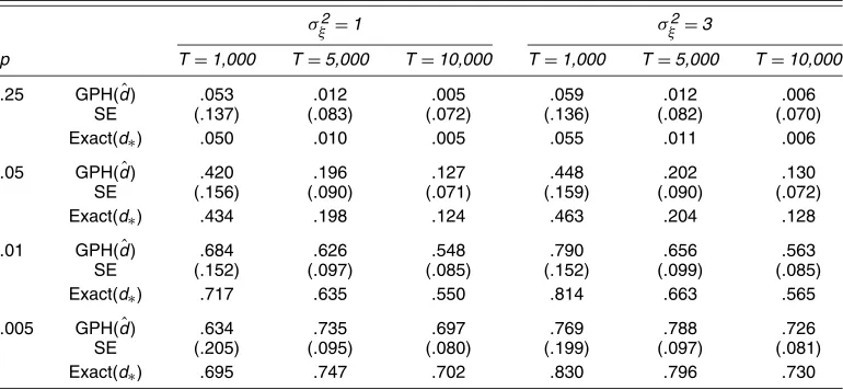
To demonstrate the GPH bias, I simulate data from the sta-tionary RLS process for various parameter settings and apply the GPH estimator using the rule-of-thumb value J=T1/2. I present the results from GPH estimation in Table 1. The rows labeled “GPH” contain the mean values ofdˆ over 1,000 Monte Carlo trials, and the rows labeled “Exact d” contain the val-uesd∗ computed from the population spectrum as in (8). The sample size,T, ranges from 1,000 to 10,000. This range cor-responds to the samples sizes that typically arise in economics and finance with data measured at weekly or daily frequencies. Forp< .05, the GPH estimator is substantially biased. In al-most all cases, however, the exact valued∗closely corresponds
Table 1. Mean Values ofd for a RLS Processˆ
σξ2=1 σξ2=3
p T=1,000 T=5,000 T=10,000 T=1,000 T=5,000 T=10,000
.25 GPH(dˆ) .053 .012 .005 .059 .012 .006 SE (.137) (.083) (.072) (.136) (.082) (.070) Exact(d∗) .050 .010 .005 .055 .011 .006
.05 GPH(dˆ) .420 .196 .127 .448 .202 .130 SE (.156) (.090) (.071) (.159) (.090) (.072) Exact(d∗) .434 .198 .124 .463 .204 .128
.01 GPH(dˆ) .684 .626 .548 .790 .656 .563 SE (.152) (.097) (.085) (.152) (.099) (.085) Exact(d∗) .717 .635 .550 .814 .663 .565
.005 GPH(dˆ) .634 .735 .697 .769 .788 .726 SE (.205) (.095) (.080) (.199) (.097) (.081) Exact(d∗) .695 .747 .702 .830 .796 .730
NOTE: The rows labeled “GPH” give the average of the GPH estimate across 1,000 realizations of sizeTfrom the RLS processyt=µt+εt, µt=(1−st)µt−1+stξt,st∼iid Bernoulli(p),ξt∼iid(0,σξ2), andεt∼N(0, 1). The GPH statistic is computed withJ=T1/2. The rows labeled
SE give the standard deviation of the GPH estimates across the 1,000 realizations. The asymptotic standard errors for Gaussian processes are .114, .076, and .064 for samples of size 1,000, 5,000, and 10,000 (see Hurvich et al. 1998). The rows labeled Exact(d*) give the GPH estimate
computed using the log spectrum in place of the log periodogram.
to the average GPH estimate. This proximity shows that d∗ dominates the GPH bias, and indicates that we can ignore the contribution of the second term in (9). Agiakloglou, Newbold, and Wohar (1993) demonstrated the same phenomenon for sta-tionary AR(1) processes.
The only case in Table 1 where the average GPH estimate deviates fromd∗is whenT=1,000 andpis very close to 0. In this case some of the Monte Carlo realizations contain no level shifts, causingdˆto be close to 0 for those realizations. However, conditional on there being at least one break in a sample, the average GPH estimate is close to d∗. This bisection leads to a bimodal distribution for dˆ, a feature that Diebold and Inoue (2001) also documented. This bimodal property results from the discontinuity in the spectrum of the process at the point where the probability of a break equals 0.
There are several other notable features in Table 1. First, as T increases, the average GPH estimate approaches 0. This convergence is not surprising, given that the dominant term in the bias, d∗, isO(J2/T2)and thus converges to 0 as T→ ∞ (see Hurvich et al. 1998, lemma 1). Second, the standard errors monotonically decrease inTin all cases. Third, the average es-timate of d increases in σξ2, the size of the level shifts. This association arises because larger shifts increase the importance of the persistentµtterm relative to the iidεtterm. However, the
effect of shift size on the GPH bias diminishes asT increases. This diminution is consistent with Theorem 1, given in the next section, which shows that shift size does not matter asymptoti-cally.
3.2 Asymptotic GPH Bias
Hurvich et al. (1998, lemma 1) showed that d∗ converges pointwise to 0 asTincreases, that is,d∗→0 as we move from left to right along the rows in Table 1. For large p, this con-vergence occurs quickly. However,d∗ can be far away from 0 whenpis small, even for largeT. Whenp=0, the value ofd∗is identically 0 for allT. Thus the pointwise limit ofd∗provides a satisfactory approximation whenp=0 and whenpis large, but
we need a better approximation whenplies in a local neighbor-hood of 0.
This problem parallels that of estimating the largest root in an autoregression when that root is near unity. Both cases involve an estimator that exhibits substantial bias in the neighborhood of a point of discontinuity. Influential work by Phillips (1988) and Cavanagh, Elliott, and Stock (1995) showed that by spec-ifying the autoregressive parameter as lying in a local neigh-borhood of unity, a better large-sample approximation to the distribution of the least squares estimator can be obtained.
Diebold and Inoue (2001) used a similar technique to ana-lyze a Markov-switching process with rare shifts. They speci-fied the switching probability within a local neighborhood of 0 and showed that the variance of partial sums is of the same or-der of magnitude as the variance of partial sums of a fraction-ally integrated process. However, this result does not admit a particular order of magnitude for the local neighborhood of 0 that containsp. Thus it implies that a Markov-switching process can be approximated by an integrated process of any nonnega-tive order, depending the chosen neighborhood. Breidt and Hsu (2002) provided similar results for the RLS process.
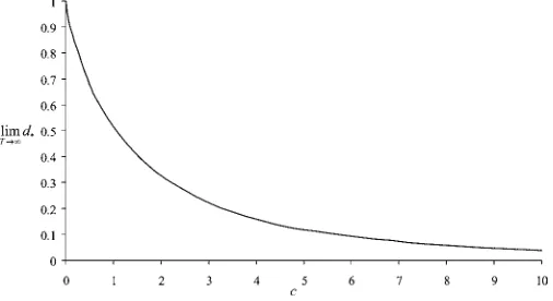
In Theorem 1 I show that the appropriate choice of neigh-borhood size depends critically onJ, the number of terms in the GPH regression. This dependence onJemanates from the denominator of the second term in the spectrum (7), which is p2+(1−p)(2−2 cos(ω))≈p2+ω2for smallω andp. By setting p to the same order of magnitude as ω, I isolate the dominant component of the spectrum. This isolation produces a good approximation tod∗for small values ofp. Specifically, it is appropriate to setpT =cJ/T, wherecis a positive
con-stant. Because var(T−1Tt=1µt)=ση2/pTT, this condition
im-plies that var(T−1Tt=1µt)=O(J−1). The following theorem
formalizes these arguments and obtains the asymptotic bias of the GPH estimator.
Theorem 1. Consider the MN process in (1) and (2) and sup-pose that fε(ω) <B0<∞,fη(ω) <B0<∞, and |fη′(ω)|<
Figure 2. Asymptotic Bias of the GPH Estimator. This curve ap-plies to data generated by yt=µt+εt,µt=(1−pT)µt−1+√pTηt,
ηt∼short memory,εt∼short memory, and t=1, 2, . . . ,T . The
band-width (number of frequencies) in the GPH regression is J=pTT/c.
B1 < ∞ for all ω in a neighborhood of 0. Assume that
where (x,s,a)denotes the Lerch transcendent function. Theorem 1 provides an approximation to the bias in the GPH estimator when a general MN process generates the data. This asymptotic bias is a function of the Lerch transcendent func-tion, also known as the Lerch zeta funcfunc-tion, which is a gener-alization of the Riemann zeta function (Gradshteyn and Ryzhik 1980, p. 1072). The only parameter in the asymptotic bias is c=pTT/J. This result indicates that the reduction in bias from
decreasing J asymptotically equals the decrease in bias from a proportionate increase in por T. Figure 2 plots the asymp-totic bias and shows that it ranges between 0 and 1 and de-creases monotonically inc. This graph emphasizes the fact that the GPH bias depends both on the properties of the data and on the specification of the estimator. One cannot say that a level-shift process appears to be fractionally integrated of some order dwithout reference to the bandwidthJ.
Theorem 1 implies thatd∗does not converge to 0 uniformly inp∈ [0,1]; that is, supp0,p1∈[0,1]d∗does not converge to 0 as
T → ∞. In other words, for every T there exists a value of psuch thatd∗>0, despite the fact thatd∗converges pointwise to 0. Thus, traveling from left to right along the rows of Table 1, d∗decreases toward 0, but there exists a path through the table in a southeast direction for whichd∗does not converge to 0.
4. MODIFIED GPH REGRESSION
As shown in Section 3, the GPH statistic may erroneously indicate long memory when the MN process generates the data. In this section I use the result in Theorem 1 to suggest a simple modification to the GPH estimator that reduces bias when the data-generating process contains level shifts. An important ad-vantage of the modified GPH estimator is its simplicity. It can be implemented easily by adding an extra regressor to the GPH regression. This straightforwardness makes it a useful diagnos-tic tool for signalling whether a fully specified model with level shifts could outperform a long-memory model.
The asymptotic bias in Theorem 1 derives from the fact that when p is small, the dominant component of the spectrum at low frequencies is−log(p2+ω2)plus a constant. This dom-inant term is nonlinear in log(ω), so adding −log(p2+ω2) as an extra regressor in the GPH regression would reduce the bias caused by level shifts. However, this strategy is infeasible, because pis unknown. I create a feasible estimator by setting pT=kJ/Tfor some constantk>0 and running the regression
The modified GPH estimator is
ˆ
dk=dk∗+(X′MZX)−1X′MZlog(fˆ/f),
where X≡X− X, MZ =I −Zk(Zk′Zk)−1Z′k,Zk≡Zk− Zk,
X=J−1Jj=1Xj,Zk=J−1Jj=1Zkj, anddk∗denotes the
esti-mator computed from the spectrum rather than from the peri-odogram. Next I derive the asymptotic properties of the modi-fied GPH estimator.
4.1 Asymptotic Properties of the Modified GPH Estimator
The MN process includes Gaussian processes as a special case. However many useful models, including RLS or Markov switching, are non-Gaussian. As discussed in Section 3, current theoretical results do not allow formal treatment of the second component of the bias for log periodogram regression with non-Gaussian data. Thus, as in Theorem 1, I focus on the dominant component of the bias,dk∗. I derive an approximation todk∗for the potentially non-Gaussian MN process.
Theorem 2. Consider the MN process in (1) and (2) and sup-pose that fε(ω) <B0<∞,fη(ω) <B0<∞, and |fη′(ω)|<
rk≡ and Li2is the dilogarithm.
The asymptotic bias of the modified GPH estimator is a func-tion of cand k. Figure 3 plots this asymptotic bias for vari-ousk, along with the asymptotic bias of the GPH estimator for comparison. The asymptotic bias equals 0 when k=c, so for everycthere exists a value ofkthat completely eliminates bias. Fork>c, the bias is positive, and for k<c, the bias is neg-ative. There are some other notable features of the asymptotic bias. First, the absolute bias of the modified GPH estimator is less than the GPH bias for allk. Second, as level shifts become more frequent (i.e., asc→ ∞), the asymptotic bias goes to 0 for allk. Third, the asymptotic bias increases ink, and it con-verges to the GPH bias in Theorem 1 ask→ ∞.
The curves in Figure 3 indicate that the modified GPH esti-mator can markedly reduce the bias in the GPH estiesti-mator due to occasional level shifts. However, such bias reduction becomes only useful if the requisite loss in precision is acceptable. To ad-dress this issue, I derive the asymptotic properties of the mod-ified GPH estimator under the alternative model of Gaussian long memory.
Theorem 3. Consider the fractionally integrated processyt=
(1−L)−dut, where {ut}is a stationary short-memory process
Figure 3. Asymptotic Bias of the Modified GPH Estimator. These curves apply to data generated by yt = µt +εt, µt =
Corollary 1. Consider the process in Theorem 3 and assume also thatJ=o(T4/5)and log2T=o(J). ThenJ1/2(dˆk−d)−→d N(0, π2/24vk).
Except for the scale factors bk andvk, the asymptotic bias
and variance expressions in Theorem 3 are the same as those of Hurvich et al. (1998) for the GPH estimator. The bias factor bk takes the values−.65,−.41,−.28,−.21, and−.15 fork=
1,2,3,4, and 5. Thus the bias of the modified GPH estimator is much smaller than the GPH bias. This bias reduction arises because the extra term in the modified GPH regression picks up some of the curvature in the log spectrum that causes bias in the GPH estimator. The variance factorvktakes the values .17, .26,
.31, .35, and .37 fork=1,2,3,4, and 5. Thus, for a givenJ, the variance of the modified GPH estimator is larger than the GPH variance. However, a suitable choice ofJ mitigates this efficiency loss.
I simulate the performance of the modified GPH estimator in two settings, the RLS process and a fractionally integrated process. I illustrate the performance of the estimator across dif-ferent values ofJfor one set of parameter values. In Section 4.2 I give results for a range of parameter values, sample sizes, and methods for choosingJ.
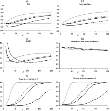
Figure 4 shows the performance of the modified GPH esti-mator as a function ofJwhen applied to a RLS process with T=5,000 andp=.02. Figures 4(a) and 4(b) shows that the as-ymptotic bias from Theorem 2 closely corresponds to the actual bias. For all values ofk, this bias is markedly lower than for the GPH estimator. Figure 4(e) also reveals the lower bias of the modified GPH estimator. It shows that a standardt-test based on the modified GPH estimate erroneously rejects the null hy-pothesis thatd=0 less often than the GPH estimator. The size of this test increases inkbecause the estimator bias increases ink. Figure 4(c) shows that the values ofJ that minimize the root mean squared error (RMSE) of the modified GPH estima-tor exceed the values ofJthat minimize the RMSE of the GPH estimator. The minimum RMSE values are similar across the values ofkand are less than those of the GPH estimator.
Figures 4(d), 4(c), and 4(f ) illustrate that the variance and as-ymptotic normality results in Theorem 3 and its corollary also apply to the RLS process. Figure 4(d) shows that the estimated standard error ofdˆk closely corresponds to the actual standard error. I measure the actual standard error as the standard devia-tion ofdˆkacross the Monte Carlo draws. The estimated standard error is computed as(π/√6)(X′MZX)−1/2, which has a
limit-ing value ofπ/√24Jvk, from Theorem 3. AsJ increases
to-ward 200, the estimated standard error becomes slightly biased downward, and the ratio of the estimated standard error to ac-tual standard error decreases toward .85. However, forJ<60, the ratio exceeds .95.
Figures 4(e) and 4(f ) show that a standardt-test rejects the null hypothesis thatd=0 with a similar frequency to a hypo-thetical test that assumes normality. The rejection frequency of
(a) (b)
(c) (d)
(e) (f)
Figure 4. Performance of the Modified GPH Estimator for an RLS Process ( GPH; k=1; k=3; k=5). The data-generating process was yt=µt+εt,µt=(1−st)µt−1+stξt, st∼iid Bernoulli(p),ξt∼iid N(0, 1),εt∼iid N(0, 1), p=.02 and T=5,000. The curves are
generated from 1,000 Monte Carlo draws as follows: (a) average estimate of d across draws; (b) from Theorem 2; (c) computed from average and variance of estimates of d across draws; (d) estimated standard error equals (π/√6)(X′MZX )−1/2, actual standard deviation equals standard deviation of estimate of d across draws; (e) proportion of rejections of null hypothesis that d=0 against d>0, nominal size=5%; (f) size computed assuming that estimate of d is normally distributed with mean and variance given by average and variance of estimates of d across draws; nominal size=5%.
this hypothetical test equals the probability that the estimate ex-ceeds the one-sided 5% critical value, assuming that the estima-tor is normally distributed. The normal approximation appears to be adequate, especially for small values ofJ.
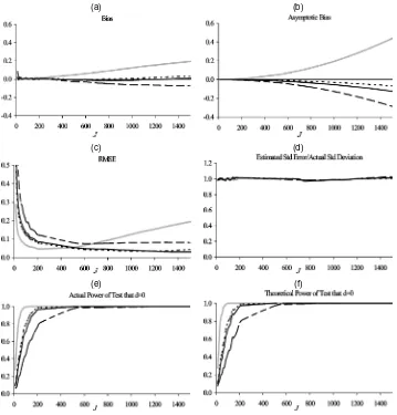
To assess the efficiency loss from the modified GPH esti-mator, I simulate from a fractionally integrated process with d=.3, where the innovations follow an AR(1) process with autoregressive parameter .4. Figure 5 presents the results for variousJ. Excluding the long-memory component, this process exhibits less dependence than the RLS process in Figure 4, so the RMSE in Figure 5 is minimized for greater values ofJthan in Figure 4. Figures 5(d), 5(e), and 5(f ) corroborate the theo-retical variance and asymptotic normality results in Theorem 3 and its corollary.
Figures 5(a) and 5(b) show that the bias of the GPH estima-tor exceeds the modified GPH bias for all k, as predicted by Theorem 3. However, for largeJ, the asymptotic bias overesti-mates the actual bias, because the second-order terms in the bias expression become nonnegligible. Furthermore, the asymptotic bias overestimates the actual bias by more for the modified GPH estimator than for the GPH estimator, which implies that the
asymptotic results overstate the finite-sample RMSE efficiency loss of the modified GPH estimator. I study this point further in Section 4.2.
4.2 ChoosingJ andk
From Theorem 3, the MSE ofdˆkfor Gaussian long memory is
MSE(dˆk)=b2k4π 4
81 f′′
u(0)
fu(0)
2J4
T4 + π2 24Jvk
+o(J4T−4)+O(JT−2log3J)+o(J−1). The value ofJthat minimizes MSE is
J=(vkb2k)−1/5
27 128π4
1/5f′′
u(0)
fu(0)
−2/5
T4/5, (10)
ignoring the remainder terms and assuming that fu′′(0)=0. The MSE-optimal value ofJ in (10) equals that for the GPH estimator (see Hurvich et al. 1998), except for the scale fac-tor (vkb2k)−1/5. This scale factor takes the values 1.69, 1.88,
2.09, 2.33, and 2.58 for k=1,2,3,4, and 5. Thus for
(a) (b)
(c) (d)
(e) (f)
Figure 5. Performance of the Modified GPH Estimator for a FI Process ( GPH; k=1; k=3; k=5). The data-generating process was yt=(1−L)−dut, where d=.3, ut=.4ut−1+εt,εt∼iid N(0, 1), and T=5,000. The curves are generated from 1,000 Monte Carlo draws
as follows: (a) average estimate of d across draws; (b) from Theorem 3; (c) computed from average and variance of estimates of d across draws; (d) estimated standard error equals (π/√6)(X′MZX )−1/2; actual standard deviation equals standard deviation of estimate of d across draws;
(e) proportion of rejections of null hypothesis that d=0 against d>0, nominal size=5%; (f) power computed assuming that estimate of d is normally distributed with mean and variance given by average and variance of estimates of d across draws, nominal size=5%.
ple, if k=3, then the MSE-optimal choice of J is approxi-mately double the MSE-optimal choice for the GPH estimator. Hurvich and Deo (1999) proposed a consistent estimator for the ratio fu′′(0)/fu(0) that enables plug-in selection of the
MSE-optimal J. Their estimator is the coefficient on.5ω2j in a regression of the log periodogram onXjand.5ωj2.
If Jequals its MSE-optimal value, then, for Gaussian long memory,
MSE(dˆk)=
|bk|
v2k 2/5
MSE(dˆ), (11)
excluding the remainder terms. Thus the RMSE of the mod-ified GPH estimator is (|bk|/v2k)1/5 times the RMSE of the
GPH estimator when J is chosen to be MSE-optimal. This scale factor takes the values 1.86, 1.44, 1.24, 1.11, and 1.02 for k=1,2,3,4, and 5. Thus, there is negligible asymptotic efficiency loss whenk=5.
The asymptotic MSE in (11) does not apply to the MN process for smallp. In this case, as shown in Theorem 2, the bias isO(1)and dominates the variance for allJ. The modified
GPH estimator often has smaller RMSE than the GPH estima-tor in this case, because the extra term in the log periodogram regression mitigates bias. Suppose that we chooseJas in (10), implying thatJincreases ink. Because the local-to-0 parameter cequalspT/J, a larger value ofJimplies a smaller value ofc. Figure 6 presents the asymptotic bias of the modified GPH esti-mator from Theorem 2, assuming thatJis chosen as in (10). Re-call that Figure 3 shows the asymptotic bias for the case when Jis fixed across values ofk. Figure 6 is the same as Figure 3, but with the curves stretched horizontally to reflect decreasing values ofcas kincreases. Figure 6 reveals negligible bias re-duction fork=5, but substantial bias reduction whenk<5.
Given a value ofJ, choosingk=cimplies that the asymp-totic bias of the modified GPH estimator equals 0. However, ccannot be efficiently estimated, because it defines a shrinking neighborhood around 0, and thus larger samples bring little in-formation about it. If one were ignorant about the value ofc, thenkcould be chosen to minimize average bias over all pos-sible values ofc. To this end, I numerically integrate under the absolute value of the asymptotic bias curves in Theorem 2, and
Figure 6. Asymptotic Bias of Modified GPH Estimator for MSE Opti-mal J ( k=1; k=3; k=5; GPH). These curves apply to data generated by yt=µt+εt,µt=(1−pT)µt−1+√pTηt,ηt∼short
memory,εt∼short memory, and t=1, 2, . . . ,T . The bandwidth
(num-ber of frequencies) in the GPH regression is J=pTT/c.
find that average bias is minimized atk=3.16;it is decreasing ink for 0 < k<3.16 and increasing in kfor 3.16 < k<∞. Because the asymptotic bias is almost identical fork=3 and k=3.16, I recommend rounding to the nearest integer and set-tingk=3.
For a given choice of J, choosing k=3 minimizes aver-age bias if the process contains rare level shifts. If we choose MSE-optimal J, thenk=3 implies a 24% higher asymptotic RMSE than for the GPH estimator if the true process contains long memory [see (11)]. However, in simulations that follow I show that the efficiency loss can be much less than 24% in
finite samples. In fact, modified GPH regression has a lower RMSE than GPH regression in some long-memory cases.
I simulate the performance of the modified GPH estimator for various parameter settings. I use both the rule-of-thumb value ofJ=T1/2and the plug-in method of Hurvich and Deo (1999) to selectJ. Results for the RLS process are presented in Table 2, and results for a fractionally integrated process are con-tained in Table 3. For plug-in selection ofJ, the results for the modified GPH estimator withk=5 closely match those for the GPH estimator. This correspondence is consistent with the as-ymptotic bias curves in Figure 6 and the similarity between the asymptotic RMSEs of each estimator. The modified GPH es-timator withk=1 can have substantially negative bias, which leads to high RMSE values in many cases.
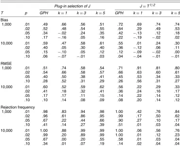
For the RLS process, setting k=3 results in the lowest RMSE whenp> .02 andJis chosen using the plug-in method. For example, ifT=10,000 andp=.05, then the RMSE when k=3 improves by 35% over the GPH estimator. The RMSE improves by 22% over GPH when p=.02 and by 20% when p=.1 for this same sample size. Size distortion also reduces substantially relative to the GPH estimator in these cases.
In the plug-in method, J increases withkaccording to the relationship in (10). This feature results in reduced RMSE for the modified GPH estimator over the GPH estimator in many cases, reinforcing the results in Figure 4. The only cases where RMSE for plug-in selection ofJexceeds that for rule-of-thumb selection occur for RLS whenpis small, which corroborates the findings of Hurvich and Deo (1999), who stated that the plug-in method works well unless the spectrum is too peaked near zero frequency.
Table 2. Properties of the Modified GPH Estimator for an RLS Process
Plug-in selection of J J=T1/2
T p GPH k=1 k=3 k=5 GPH k=1 k=3 k=5
Bias
1,000 .01 .49 .66 .56 .51 .72 .69 .74 .74
.02 .52 .48 .54 .55 .64 .29 .49 .53
.05 .34 −.02 .24 .35 .42 −.13 .12 .18
.10 .17 −.16 .05 .16 .22 −.19 −.02 .02 10,000 .01 .59 .47 .58 .61 .55 .01 .24 .30
.02 .40 .05 .30 .40 .36 −.12 .06 .11
.05 .15 −.10 .05 .12 .12 −.09 −.02 .00
.10 .06 −.07 −.01 .03 .04 −.04 −.01 −.01 RMSE
1,000 .01 .51 .74 .58 .54 .71 .91 .81 .80
.02 .54 .66 .58 .57 .66 .63 .60 .61
.05 .40 .50 .38 .41 .45 .53 .34 .33
.10 .28 .52 .31 .29 .26 .56 .31 .27 10,000 .01 .60 .52 .59 .62 .56 .22 .29 .33
.02 .41 .18 .32 .41 .36 .24 .16 .17
.05 .17 .17 .11 .15 .14 .22 .14 .12
.10 .10 .14 .08 .09 .08 .20 .14 .12 Rejection frequency
1,000 .01 .98 .83 .94 .98 1.00 .42 .76 .84
.02 .96 .61 .86 .95 .99 .17 .50 .62
.05 .67 .22 .44 .66 .90 .27 .10 .17
.10 .41 .14 .27 .39 .51 .01 .03 .04 10,000 .01 1.00 .88 .99 .99 1.00 .06 .56 .76
.02 .99 .20 .89 .99 1.00 .01 .12 .23
.05 .67 .00 .20 .55 .58 .01 .03 .04
.10 .34 .01 .07 .19 .14 .02 .04 .04
NOTE: The data-generating process wasyt=µt+εt,µt=(1−st)µt−1+stξt,st∼iid Bernoulli(p),ξt∼iid N(0, 1),εt∼iid N(0, 1).
The elements in the table are averages across 1,000 Monte Carlo realizations. The plug-in method was used withL=.1T6/7frequencies in
first-stage regression.
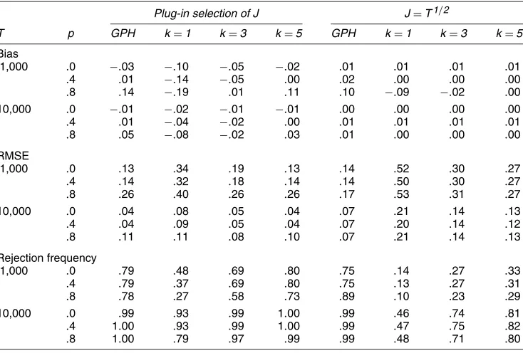
Table 3. Properties of the Modified GPH Estimator for a Fractionally Integrated Process
Plug-in selection of J J=T1/2
T p GPH k=1 k=3 k=5 GPH k=1 k=3 k=5
Bias
1,000 .0 −.03 −.10 −.05 −.02 .01 .01 .01 .01
.4 .01 −.14 −.05 .00 .02 .00 .00 .00
.8 .14 −.19 .01 .11 .10 −.09 −.02 .00 10,000 .0 −.01 −.02 −.01 −.01 .00 .00 .00 .00
.4 .01 −.04 −.02 .00 .01 .01 .01 .01
.8 .05 −.08 −.02 .03 .01 .00 .00 .00 RMSE
1,000 .0 .13 .34 .19 .13 .14 .52 .30 .27
.4 .14 .32 .18 .14 .14 .50 .30 .27
.8 .26 .40 .26 .26 .17 .53 .31 .27 10,000 .0 .04 .08 .05 .04 .07 .21 .14 .13
.4 .04 .09 .05 .04 .07 .20 .14 .12
.8 .11 .11 .08 .10 .07 .21 .14 .13 Rejection frequency
1,000 .0 .79 .48 .69 .80 .75 .14 .27 .33
.4 .79 .37 .69 .80 .75 .13 .27 .31
.8 .78 .27 .58 .73 .89 .10 .23 .29 10,000 .0 .99 .93 .99 1.00 .99 .46 .74 .81
.4 1.00 .93 .99 1.00 .99 .47 .75 .82
.8 1.00 .79 .97 .99 .99 .48 .71 .80
NOTE: The data-generating process wasyt=(1−L)−dut, whered=.3,ut=put−1+εt, andεt∼iid N(0,1). The elements in the table
are averages across 1,000 Monte Carlo realizations. The plug-in method was used withL=.1T6/7frequencies in first-stage regression.
For the long-memory process withp=.8, the modified GPH estimator with k=3 outperforms the GPH estimator. It has a smaller bias and RMSE. Thus the modified GPH estimator has the power to correct bias caused by pure autoregressive processes. When the short-memory component is less persis-tent (p=0 andp=.4), the RMSE of the modified GPH esti-mator slightly exceeds that for the GPH estiesti-mator. In summary, the modified GPH estimator withk=3 andJselected using the plug-in method performs well in most settings.
4.3 Applications
To illustrate the modified GPH estimator, I apply it to the weekly relative price of soybeans to soybean oil and to daily
volatility in the S&P 500. The soybean price data span Janu-ary 1, 1953 to June 30, 2001 and contain the average weekly soybean price in central Illinois and the average weekly soy-bean oil price in Decatur, Illinois. There are a total of 2,455 ob-servations. Given that soybean oil derives from soybeans, the prices of these two commodities should have a common trend, which implies that the ratio of their prices should be mean-reverting. Figure 7(a) plots the log relative price series and indi-cates that it is mean-reverting with strong positive dependence. This structure suggests that potential candidate models for the relative price include long memory and short memory with level shifts.
Table 4 presents the estimated values of d from the GPH and modified GPH estimators. The estimated value of d for
(a) (b)
Figure 7. Soybean and S&P 500 Time Series. (a) Log relative price of soybeans and soybean oil; (b) absolute daily returns on the S&P 500. The soybean data span January 1, 1953 to June 30, 2001 and contain the average weekly soybean price in central Illinois and the average weekly soybean oil price in Decatur, Illinois. There are a total of 2,455 observations, and the units of measurement are cents per bushel for soybeans and cents per pound for soybean oil. The S&P 500 data span January 1, 1961 to July 31, 2002 and comprise the absolute daily returns on the S&P 500 stock index. There are a total of 10,463 observations.
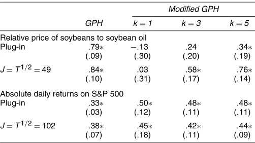
Table 4. Estimates of the Long-Memory Parameter
Modified GPH
GPH k=1 k=3 k=5
Relative price of soybeans to soybean oil
Plug-in .79∗ −.13 .24 .34∗ (.09) (.30) (.20) (.19)
J=T1/2=49 .84∗ .03 .58∗ .76∗
(.10) (.31) (.17) (.14) Absolute daily returns on S&P 500
Plug-in .33∗ .50∗ .48∗ .48∗ (.03) (.12) (.11) (.11)
J=T1/2=102 .38∗ .45∗ .42∗ .44∗
(.07) (.18) (.11) (.09)
NOTE: The cells contain estimates ofd, the long-memory parameter, with standard errors below each estimate in parentheses.∗indicates significance at 5%, using standard normal critical values and a one-sided alternative. The soybean data span January 1, 1953 to June 30, 2001 and contain the average weekly soybean price in central Illinois and the average weekly soybean oil price in Decatur, Illinois. There are a total of 2,455 observations. The stock market data span January 1, 1961 to July 31, 2002 and contain the absolute daily returns on the S&P 500 stock index. There are a total of 10,463 observations. The plug-in method was used with
L=.1T6/7frequencies in first-stage regression. The estimated plug-in value ofJfor the GPH
estimator are 67 for soybeans and 657 for the S&P 500. The plug-in values ofJfor the modified GPH estimator equal the scale factors in (10) multiplied by 67 (for soybeans) and 657 (for the S&P 500).
the soybean data equals .79 when the plug-in method is used to select J and .84 when J=T1/2. These values are signifi-cantly different from 0. The modified GPH estimates are sub-stantially smaller than the GPH estimates for both methods of bandwidth selection. When the plug-in selection method is used withk=3, the estimate ofd equals .24 and is insignificantly different from zero. Whenk=1, the estimated value of d is also insignificant. Thus a short-memory model with level shifts is a viable alternative to long memory for these data.
Liu (2000), Granger and Hyung (1999), Lobato and Savin (1998), and others have cited financial market volatility as one setting in which long memory and level shifts provide compet-ing model specifications. I apply the modified GPH estimator to absolute daily returns on the S&P 500. The data are plotted in Figure 7(b). The sample period is January 1, 1961 to July 31, 2002, and returns are measured as the log price change. Table 4 indicates that a short-memory model with level shifts is not a viable alternative to long memory for this series. In fact, the modified GPH estimates exceed the GPH estimates for all val-ues ofJandk. The GPH estimates are .33 and .38 for the two methods of choosingJ, whereas the modified GPH estimates range from .42 to .50. This result is not sensitive to the measure of volatility; using squared returns and the log of absolute re-turns leads to same conclusion. Thus long memory in volatility of S&P 500 returns appears to not be illusory.
5. CONCLUSION
This article has addressed the illusion of fractional integra-tion, or long memory, in time series containing level shifts. I have focused on the GPH estimator, which is used liberally in empirical work. When applied to a short-memory MN process, the GPH estimator is biased and often erroneously indicates the presence of long memory. I have derived a large-sample approx-imation to this bias and used it to formulate a new estimator that has markedly smaller bias. I illustrated the modified GPH
estimator with applications to the relative price of soybeans to soybean oil and to stock market volatility.
The modified GPH estimator requires choosing a value for a nuisance parameter k. This parameter proxies for a local-to-0 parameter that cannot be well estimated from the data. I rec-ommend settingk=3, which minimizes average absolute bias across all possible values of the true parameterc. For a given bandwidthJ, this recommendation leads to positive bias in the modified GPH estimator if c<3 and negative bias if c>3. Despite this trade-off, the modified GPH estimator withk=3 exhibits less absolute bias than the original GPH estimator for all values of c(see Figs. 3 and 6). Thus, although it does not completely eliminate bias due to level shifts, the modified GPH estimator with k=3 significantly reduces bias relative to the GPH estimator.
The modified GPH estimator suggests whether a short-memory model with level shifts should be considered as an alternative to long memory. It is based on the spectrum, which represents the linear dependence properties of a time series. However, a process with discrete level shifts has a nonlinear dependence structure, because the innovations that define break points are much more persistent than other innovations. Models that capture this nonlinearity will generate more accurate infer-ence about the features of the data than can be achieved with estimators such as modified GPH.
Specifying models that identify the persistent innovations in a time series is nontrivial, especially given that each of these shocks may have a different origin. They may arise from a political event, a weather event, a war, a new technology, an earnings announcement, or a government policy change, to name a few possibilities. Most Markov-switching models, and the particular STOPBREAK model of Engle and Smith (1999), take an agnostic approach and focus only on the time series characteristics of the data when identifying break points. However, Filardo (1994) and Filardo and Gordon (1998) es-timated Markov-switching models that use observed data to help identify break points. Further research in this vein will improve model performance and enable better discrimination between models with occasional persistent shocks and linear long-memory models.
ACKNOWLEDGMENTS
The author is a member of the Giannini Foundation of Agricultural Economics. He thanks Oscar Jorda, Prasad Naik, Doug Steigerwald, the editor, an associate editor, and an anony-mous referee for suggestions and comments that improved the quality of this article.
APPENDIX: PROOFS Proof of Theorem 1
Recall thatpT=cJ/T. We can decompose log(fj)as
logfj=log
fε(ωj)+
pT
p2T+(1−pT)(2−2 cos(ωj))
fη(ωj)
= −log(1+p−T2ω2j)
+log
The results from Hurvich and Beltrao (1994),
|Xj− X| =O(logJ)=O(logT),
where (x,s,a) denotes the Lerch transcendent function (Gradshteyn and Ryzhik 1980, p. 1072).
For the second term in (A.1), note that|fη(ωj)−fη(ω˜J)| ≤
Proof of Theorem 2
From the proof of Theorem 1, we have
J
where (x,s,a) denotes the Lerch transcendent function (Gradshteyn and Ryzhik 1980, p. 1072).
Note that
The log spectrum of the fractionally integrated process is logfj=dXj+logfuj. Thus the modified GPH estimator is
ˆ
dk=d+(X′MZX)−1X′MZlogfu
+(X′MZX)−1X′MZlog(ˆf/f), (A.2)
whereX=X− X,MZ=I −Zk(Zk′Zk)−1Zk′, andZk=Zk− Zk.
Consider the second term on the right side of (A.2). We have
X′MZlogfu
whererk is as defined in the proof of Theorem 2. From
Hur-vich et al. (1998), a second-order expansion offuaroundω=0
yields
where Kj is bounded uniformly in j for sufficiently large T.
Given this, Hurvich et al. (1998) showed that
J
wherefu′′denotes the second derivative offu. Similarly, J
Now, using arguments from the proof of Theorem 2, we have
J−1
Then the second term on the right side of (A.2) is
(X′MZX)−1X′MZlogfu= −bk
andvkis as defined in the proof of Theorem 2.
For the last term in (A.2), I use the proof of lemma 8 of Hurvich et al. (1998). Their proof goes through if their aj=Xj− Xis replaced by((Xj− X)−rk(1+o(1))(Zkj− Zk))
and their 2Sxx is replaced by 4Jvk(1+o(1)). These
replace-ments are valid, because the substituted terms are of the same order of magnitude as their replacements. It follows that (X′MZX)−1X′MZE(log(fˆ/f))=O(log3J/J). Thus the bias is
For the variance, I use the proof of theorem 1 of Hurvich et al. (1998). Replacing theiraj by ((Xj− X)−rk(1+o(1))(Zkj−
This result follows directly from Theorems 2 and 3 herein and theorem 2 of Hurvich et al. (1998), with theiraj replaced
by((Xj− X)−rk(1+o(1))(Zkj− Zk))and their 2Sxxreplaced
by 4Jvk(1+o(1)).
[Received January 2003. Revised May 2004.]
REFERENCES
Agiakloglou, C., Newbold, P., and Wohar, M. (1993), “Bias in an Estimator of the Fractional Difference Parameter,”Journal of Time Series Analysis, 14, 235–246.
Bai, J., and Perron, P. (1998), “Testing for and Estimation of Multiple Structural Changes,”Econometrica, 66, 47–79.
Breidt, F. J., and Hsu, N. J. (2002), “A Class of Nearly Long-Memory Time Series Models,”International Journal of Forecasting, 18, 265–281. Cavanagh, C. L., Elliott, G., and Stock, J. H. (1995), “Inference in Models With
Nearly Integrated Regressors,”Econometric Theory, 11, 1131–1147. Chen, C., and Tiao, G. C. (1990), “Random Level-Shift Time Series Models,
ARIMA Approximations, and Level-Shift Detection,”Journal of Business & Economic Statistics, 8, 83–97.
Chib, S. (1998), “Estimation and Comparison of Multiple Change-Point Mod-els,”Journal of Econometrics, 86, 221–241.
Deo, R. S., and Hurvich, C. M. (2001), “On the Log Periodogram Regression Estimator of the Memory Parameter in Long-Memory Stochastic Volatility Models,”Econometric Theory, 17, 686–710.
Diebold, F. X., and Inoue, A. (2001), “Long Memory and Regime Switching,”
Journal of Econometrics, 101, 131–159.
Engle, R. F., and Smith, A. D. (1999), “Stochastic Permanent Breaks,”Review of Economics and Statistics, 81, 553–574.
Filardo, A. J. (1994), “Business Cycle Phases and Their Transitional Dynam-ics,”Journal of Business & Economic Statistics, 12, 299–308.
Filardo, A. J., and Gordon, S. (1998), “Business Cycle Durations,”Journal of Econometrics, 85, 99–113.
Geweke, J., and Porter-Hudak, S. (1983), “The Estimation and Application of Long-Memory Time Series Models,”Journal of Time Series Analysis, 4, 221–238.
Gradshteyn, I. S., and Ryzhik, A. D. (1980),Table of Integrals, Series, and Products: Corrected and Enlarged Edition, New York: Academic Press. Granger, C. W. J. (1981), “Some Properties of Time Series Data and Their Use
in Econometric Model Specification,”Journal of Econometrics, 16, 121–130. Granger, C. W. J., and Ding, Z. (1996), “Varieties of Long-Memory Models,”
Journal of Econometrics, 73, 61–77.
Granger, C. W. J., and Hyung, N. (1999), “Occasional Structural Breaks and Long Memory,” Discussion Paper 99-14, University of California, Dept. of Economics.
Granger, C. W. J., and Joyeux, N. (1980), “An Introduction to Long-Memory Time Series Models and Fractional Differencing,”Journal of Time Series Analysis, 1, 15–39.
Hamilton, J. D. (1989), “A New Approach to the Economic Analysis of Non-stationary Time Series and the Business Cycle,”Econometrica, 57, 357–384. (1994), Time Series Analysis, Princeton, NJ: Princeton University Press.
Hidalgo, J., and Robinson, P. M. (1996), “Testing for Structural Change in a Long-Memory Environment,”Journal of Econometrics, 70, 159–174. Hurvich, C. M., and Beltrao, K. I. (1994), “Automatic Semiparametric
Estima-tion of the Memory Parameter of a Long-Memory Time Series,”Journal of Time Series Analysis, 15, 285–302.
Hurwich, C. M., and Deo, R. (1999), “Plug-in Selection of the Number of Frequencies in Regression Estimates of the Memory Parameter of a Long-Memory Time Series,”Journal of Time Series Analysis, 20, 331–341.
Hurvich, C. M., Deo, R., and Brodsky, J. (1998), “The Mean Squared Error of Geweke and Porter-Hudak’s Estimator of the Memory Parameter of a Long-Memory Time Series,”Journal of Time Series Analysis, 19, 19–46. Hurst, H. E. (1951), “Long-Term Storage Capacity of Reservoirs,”Transactions
of the American Society of Civil Engineers, 116, 770–799.
Liu, M. (2000), “Modeling Long Memory in Stock Market Volatility,”Journal of Econometrics, 99, 139–171.
Lobato, I. N., and Savin, N. E. (1998), “Real and Spurious Long-Memory Prop-erties of Stock Market Data,”Journal of Business & Economic Statistics, 16, 261–268.
McCulloch, R. E., and Tsay, R. S. (1993), “Bayesian Inference and Prediction for Mean and Variance Shifts in Autoregressive Time Series,”Journal of the American Statistical Association, 88, 968–978.
Phillips, P. C. B. (1988), “Regression Theory for Near-Integrated Time Series,”
Econometrica, 56, 1021–1043.
Timmermann, A. (2001), “Structural Breaks, Incomplete Information, and Stock Prices,”Journal of Business & Economic Statistics, 19, 299–314. Velasco, C. (2000), “Non-Gaussian Log Periodogram Regression,”
Economet-ric Theory, 16, 44–79.