Full Terms & Conditions of access and use can be found at
http://www.tandfonline.com/action/journalInformation?journalCode=ubes20
Download by: [Universitas Maritim Raja Ali Haji] Date: 12 January 2016, At: 23:28
Journal of Business & Economic Statistics
ISSN: 0735-0015 (Print) 1537-2707 (Online) Journal homepage: http://www.tandfonline.com/loi/ubes20
Comment
Yacine Aït-Sahalia, Per A Mykland & Lan Zhang
To cite this article: Yacine Aït-Sahalia, Per A Mykland & Lan Zhang (2006) Comment, Journal of Business & Economic Statistics, 24:2, 162-167, DOI: 10.1198/073500106000000152
To link to this article: http://dx.doi.org/10.1198/073500106000000152
Published online: 01 Jan 2012.
Submit your article to this journal
Article views: 46
View related articles
Comment
Yacine A
ÏT-S
AHALIADepartment of Economics and Bendheim Center for Finance, Princeton University, and NBER, Princeton, NJ 08544-1021 (yacine@princeton.edu)
Per A. M
YKLANDDepartment of Statistics, The University of Chicago, Chicago, IL 60637 (mykland@galton.uchicago.edu)
Lan Z
HANGDepartment of Finance, University of Illinois at Chicago, Chicago, IL 60607 (lanzhang@uic.edu)
We enjoyed reading the article by Hansen and Lunde (HL thereafter), and are pleased to be able to contribute some com-ments. We raise some issues that we feel are important. Some of them are addressed in our own work, and others are open questions. We certainly believe that this is an important area that will see substantial development over the next few years.
1. COVARIATION BETWEEN THE EFFICIENT PRICE AND THE NOISE
Exploring a possible correlation between the efficient price and the noise, as HL do, is an exciting and challenging task. By examining the volatility signature plots of trades and quotes, HL report that realized variance (RV) estimates based on quotes at very high frequency decrease. This is different from many earlier findings on volatility signature plots based on transaction prices. It is important to figure out how much of that is driven by the preprocessing of the data of HL, and we discuss the role that this might have played in delivering that result.
A different issue is that volatility signature plots give us a point estimate of RV at different sampling frequencies. A sub-stantial increase or decrease of RV at high sampling frequencies can signify an upward bias or downward bias. But what magni-tude of change in RV is large enough to be considered a signal for bias? This can be answered by superimposing the pointwise interval estimates of RV on the original plot. It seems that HL attempt to address this issue by providing a 95% confidence band of RV(ACNW1 tick)
30. However, the 95% confidence band that
they provide, seems to represent the variation between ask, bid, and trades, rather than displaying the uncertainty in the estima-torRV(ACNW1 tick)
30 itself. In other words, we do not know whether
or not the dipping at the higher sampling frequency in HL’s fig-ure 1 is statistically significant. We know that the inconsistent estimatorRV(ACNW1 tick)
k would have a nonnegligible bias and sto-chastic term, and thus the pointwise confidence intervals could be quite wide. We explore this further here (see Table 1). We also explore the connection between this finding and the identi-fiability, or lack thereof, of certain noise models.
2. IDENTIFIABILITY, CONSISTENCY, AND EFFICIENCY
It is important at this point to remind ourselves what the ra-tionale is for (nonparametrically) estimating certain quantities on the basis of high-frequency data. The rationale is that these
quantities, such as volatility within a fixed time period (say, 1 day) can be computed with great precision. This is the case when there is no microstructure noise, as discussed by Jacod (1994) and Jacod and Protter (1998), when the asymptotic dis-tribution can be found in great generality (for specific exam-ples, see Zhang 2001; Barndorff-Nielsen and Shephard 2002). But if, for whatever reason, one cannot find precise estimates of volatility for a given day, then one is probably better off using a more parametric approach, for example, modeling the inter-day and/or intrainter-day behavior, using a generalized autoregres-sive conditional heteroscedasticity model or in continuous time dealing with the noise as done by Aït-Sahalia, Mykland, and Zhang (2005a).
So what are the desirable (asymptotic) properties in an esti-mator? There are various ways to spell out this requirement. One is consistency, which says that with enough data, the volatility (say) can be closely estimated with the estimator at hand. An even more basic requirement on the model is iden-tifiability, which says that there exists some estimator that is consistent. Finally, there isefficiency, which means that one is making good use of the data at hand.
Unfortunately, the estimators that HL use are not consistent as recognized by Zhou (see Zhou 1996, p. 47; 1998, p. 114). Of course, perhaps consistency is not an absolute requirement; one could imagine situations where an estimator is inconsistent but has only a small error. For the Zhou estimators used by HL, however, Table 1 documents that the lack of consistency does generate substantial estimation errors.
Because their estimator is inconsistent, HL focus instead on unbiasedness and asymptotic unbiasedness. It is, of course, de-sirable that an estimator be approximately unbiased, but one should be aware that the property of unbiasedness alone can guarantee very little in some cases. As an extreme example, suppose that (in the absence of noise) log prices have constant drift and diffusion coefficients,dpt=µdt+σdWt. In this case
E[(pT−p0)/T] =µ, but the unbiased estimator(pT−p0)/Tis
hardly a good approximation forµ. In fact, this estimator over any finite time spanTremains constant, irrespective of how fre-quently sampling occurs. Thus, results such as corollary 1, must be taken cautiously, because they could indicate little about our
In the Public Domain Journal of Business & Economic Statistics April 2006, Vol. 24, No. 2 DOI 10.1198/073500106000000152
Table 1. RMSE for Three Estimators
Number of observations m
100 1,000 2,000 5,000 10,000
λ=1%
Standard RV 200% 2,000% 4,000% 10,000% 20,000%
Zhou’s one-step corrected RV 28.3% 89.4% 126.5% 200.0% 282.8%
Two scales RV 21.4% 14.6% 13.0% 11.1% 9.9%
λ=.5%
Standard RV 100% 1,000% 2,000% 5,000% 10,000%
Zhou’s one-step corrected RV 14.4% 44.7% 63.2% 100.0% 141.4%
Two scales RV 17.0% 11.6% 10.3% 8.8% 7.9%
NOTE: This table reports the RMSE as a fraction of IV to first order asymptotically.λis the noise-to-signal ratio, andmis the sample size. For simplicity, it is assumed for the purpose of this calculation thatσ2is constant. For the standard RV estimator, the RMSE is 2mλ(the bias
is the dominant quantity); for Zhou’s one-step corrected RV, it is (8m)1/2λ; and for our TSRV estimator, it is 961/6m−1/6λ1/3.
ability to precisely estimate the quantity of interest. This is also the case for the results in HL’s section 4.1.
We should also note that HL’s theory does not allow for a leverage effect, that is, a correlation between the Brownian motions driving the asset price and that driving its stochas-tic volatility, which is substantial empirically (of the order of −.75). But for this, one needs the machinery of stochastic calculus; Zhang, Mykland, and Aït-Sahalia (2005b) and Zhang (2004) have explored its application to this problem. The same goes, to some extent, for the issue of allowing for a drift term, µtdt, in the efficient price.
In the cases of independent noise and noise with dependence in tick time, the volatility is identifiable even though HL’s es-timators are inconsistent. On the other hand, the volatility un-der the assumption that noise and efficient price are dependent seems to not be identifiable, as in the development immediately after corollary 1. In other cases the lack of consistency could also mask the lack of identifiability, as in section 4.1. We elab-orate more on identifiability in the next section.
Note that by using the methodology introduced by Zhang et al. (2005b), including a semimartingale model for the σt process and the device of lettingk→ ∞at an appropriate rate, the estimator of Zhou (1996, 1998) can be improved to be con-sistent. A standard error for such an estimator can presumably be found by mimicking the methods that we developed in our two-scales article (Zhang et al. 2005b). This is recognized by HL (sec. 4.2), but, unfortunately, they do not use this or any other consistent version in their analysis, nor do they compute the variance of the estimator that would result.
3. IDENTIFIABLE NOISE MODELS
In principle, one could build a complex model to relate mi-crostructure noise to the efficient price. In practice, however, separating the signal from the noise is not that simple. There are several difficult issues concerning how to model the noise. First of all, the noise can be distinguished from the efficient price only under fairly careful modeling. In most cases, the assump-tion that the noise is staassump-tionary, alone, as in HL’s assumpassump-tion 2, is not enough to make the noise identifiable. For example, we could write down an additive model for the observed (log) price process{pt}as
pti,m=p∗ti,m+uti,m,
and letp∗t andutdenote signal and noise. But this model does not guarantee that one can disentangle the signal or the volatil-ity of the signal. To see this, suppose that the efficient price can be written as
dp∗t =µtdt+σtdWt,
where the drift coefficient µt and the diffusion coefficient σt can be random and Wt is a standard Brownian motion. If we assume thatutis also an Itô process, say
dut=νtdt+γtdBt,
thenptis also an Itô process of the form
dpt=(µt+νt)dt+ωtdVt,
where ωt2 = σt2 +γt2 +2σtγtdW,Bt/dt by the Kunita– Watanabe inequality (see, e.g., Protter 2004).
Therefore, unless one imposes additional constraints, it is not possible to distinguish signal and noise in this model, and the integrated variance (quadratic variation) of the process should be taken to be0Tω2tdt. One could, of course, requireµt=0, as was done by Aït-Sahalia et al. (2005a), but estimability is pos-sible only asT→ ∞and given a parametric or similar model. Note that HL makes the assumption that the drift in the efficient price is zero. This assumption is necessary for their unbiased-ness considerations, but for the purposes of asymptotics in a fixed time interval,T, such as a day, it does not matter, for the same reason that a consistent separation of efficient price is not possible in a fixed time interval as long as the noise is also an Itô process.
The same statement, broadly interpreted (i.e., replace the in-tegrated volatility of any processXwith its quadratic variation), holds true for general semimartingales (see Jacod and Shiryaev 2003, thm. I.4.47, p. 42). One can, in some cases, extend the concept of quadratic variation to nonsemimartingales, such as the process discussed in HL’s section 4.1, see (1) later in this section. As we explain, even in this case the noise is not sepa-rable from the signal except under additional assumptions.
Therefore, we tentatively conclude that the development just after HL’s corollary 1 mostly holds for models where one can-not, in fact, distinguish signal and noise. (Corollary 1 in itself is more general, but does not address identifiability.)
What makes this problem particularly difficult is that a sub-stantial fraction of continuous processes of interest here are Itô processes, many of which have a stationary solution. One can
easily construct a stationary diffusion process with given mar-ginal distribution and exponential autocorrelation function. By superposition, and by taking limits, one can, for example, con-struct a Gaussian Itô process with mean 0 and any autocovari-ance function of the formπ(s)=0∞e−usν(du), whereνis any finite measure on[0,∞).
The only case in which one can hope to distinguish between efficient price and noise is if the noiseutis not an Itô process. One way for this to occur is if theut’s are independent for differ-entt, and hence the autocovariance function satisfiesπ(s)=0 fors=0. This is the model given in HL’s section 3.
It should be emphasized that consistency is not guaranteed if the noise is not a semimartingale. This is the case for the noise used in HL’s section 4.1. To see this, assuming that the functionψis sufficiently smooth, by Itô’s formula,
u(t)=B(t)ψ (0)−B(t−θ0)ψ (θ0)+ t
t−θ0
B(s)ψ′(t−s)ds,
(1)
and the time-lagged Brownian motion precludes semimartin-galeness (see, e.g., definition I.4.21 of Jacod and Shiryaev 2003). Consistency does not follow even in this case. Assuming that ψ (0)=ψ (θ0), one can estimate this quantity along with
the integrated volatility.
4. INFERENCE IN TICK TIME
All of the aforementioned difficulties go away if one assumes that ut is independent for differentt’s and independent of the efficient price. Because this is an overly restrictive assumption, both HL (in sec. 4.2) and ourselves (in Aït-Sahalia et al. 2005b) have fallen back on modeling dependence in tick time. The way this works is that if ti is tick numberi, one assumes that the processuti is stationary and lets the autocovariance function be given by π(k)=cov(uti,uti+k). As discussed both here and in earlier work (Aït-Sahalia et al. 2005b), this provides a scheme for obtaining reasonable estimates of the integrated volatility of the efficient price.
From a conceptual standpoint, it also makes sense to sample in tick time, because this permits sampling to adapt to the ac-tivity of the market. For transactions, it is also natural to think of the stock price as being a measurement of the efficient price and, as such, subject to measurement error just like any other measurement.
The situation with bid and ask quotes is more complex. As HL note, taking every adjustment as a tick will result in un-derstating the volatility by a factor of about 1/√2, and it may be better to take the transaction times as the tick times, even when dealing with quote data. This issue may be part of what leads to falling estimates of volatility at very high frequencies, it should not affect the analysis of transaction data, however. This does not, of course, preclude that correlation between sig-nal and noise can exist.
An issue of a perhaps rather academic nature comes up in connection with the modeling of dependency (within the noise and between noise and signal). This appears to require a tri-angular array formulation; as ticks become more frequent, so does the dependence occur over ever smaller clock time inter-vals. This is particularly so for HL’s definition of correlation,
which is given only as a limit, and it is not quite clear how to set up a model (even a triangular array model) to achieve such an effect.
Triangular array formulation is a valid and time-honored way of asymptotically capturing phenomena that would otherwise be unavailable in the limit. One of the more well-known in-stances of this is the “local to unity” asymptotics in an autore-gressive process. But here is a second worry that pertains to the signal–noise correlation found by the authors. The data them-selves do not live on a triangular array. The conceptual intent of triangular array asymptotics would seem to preclude its use on different sampling frequencies in this same dataset. The defini-tion in theorem 2 requires that the magnitude ofei,nincreases as the tick frequency increases. This framework is clearly plausi-ble when used for different frequencies in different datasets, but it is hard to believe that this occurs as the sampling frequency increases in these given datasets. There is a problem of mod-eling here that seems to be an open question for researchers to address.
5. SOME COMMENTS ON THE EMPIRICAL ANALYSIS
The article analyzes a vast amount of empirical data, the returns on the 30 Dow Jones Industrial Average stocks over the 5 years 2000–2004, including an interesting cointegration analysis. To better understand how different estimators behave, we looked at a small subset of the HL data, which was kindly made available to us: the first stock in the sample (Alcoa, ticker symbol AA) and 1 month (January 2004). Clearly, any conclu-sions drawn from such a limited analysis are to be taken with some caution, but it is certainly possible for the patterns to hold more generally.
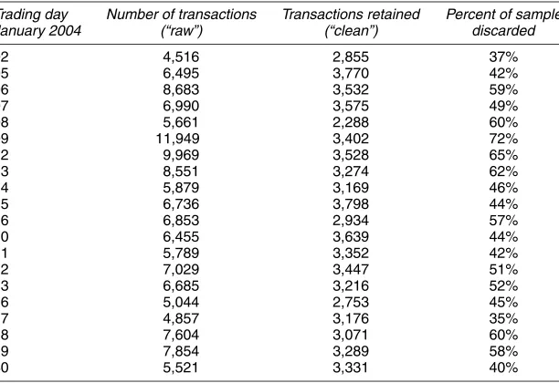
Our first concern is the degree of preprocessing of the data that HL performed, before any estimator being applied. As Ta-ble 2 shows, HL on average create a “clean” set of transactions by discarding about half of the starting sample (“raw”). In light of the percentage of the number of transactions being deleted, we are no longer talking about a light-touch cleaning of the data, but rather major surgery on the data! As we discuss later, this is not without consequences.
We downloaded the raw data for AA in January 2004 di-rectly from the TAQ database. For this particular stock and month, no transaction prices were reported at 0, and this particular sample appears to be free of major data entry er-rors. Discarding all price bouncebacks of magnitude .5% or greater eliminated fewer than 10 observations each day. [In earlier work (Aït-Sahalia et al. 2005b), we define a “bounce-back” as a log-return from one transaction to the next that is both greater in magnitude than an arbitrary cutoff, and is followed immediately by a log-return of the same magnitude but of the opposite sign, so that the price returns to its start-ing level before that particular transaction.] Thus a minimal amount of data cleaning would discard a very tiny percent-age of the raw transactions. In contrast, HL conducted their empirical analysis after eliminating transactions on the follow-ing basis: (a) deletfollow-ing ex-ante all observations originatfollow-ing from regional exchanges while retaining only those originating on the NYSE, (b) aggregating all transactions time-stamped to the
Table 2. Transactions on AA Stock, January 2004
Trading day Number of transactions Transactions retained Percent of sample January 2004 (“raw”) (“clean”) discarded
02 4,516 2,855 37%
NOTE: The table reports the number of transactions of AA stock for each trading day in January 2004. The column labeled “raw” reports the number of transactions that occurred between 9:30AMand 4:00PMEST, obtained from the TAQ database. The column labeled “clean” reports the number of transactions retained for HL’s empirical analysis. The last column reports the percentage of transactions from the raw data that are discarded when going to the clean dataset that is used for the empirical analysis in the article.
same second, and (c) eliminating transactions that appear to have taken place outside a posted bid/ask spread at the same time stamp.
Our view is that those unpleasant data features are precisely what any estimator that is robust to microstructure noise should deal with, without prior intervention. Perhaps those transactions time-stamped to the same second did not occur exactly in that order, especially if they occurred on different exchanges; per-haps the regional exchanges are less liquid or less efficient at providing price discovery, but still provide meaningful infor-mation as to the volatility of the price process for someone contemplating a trade there; perhaps the depth of the quotes is insufficient to fulfill the order, and the transaction has a nonnegligible price impact; or perhaps the matching of the quotes to the transactions that is used to eliminate transactions (which in their vast majority did actually take place) is not per-fect. In the end, this is what market microstructure noise is all about!
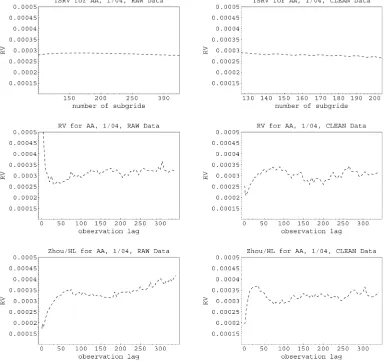
Figure 1 examines the consequences of this preprocessing of data. The left column in the figure shows the results using the “raw” data (after eliminating bouncebacks), whereas the right column uses the HL “clean” sample. The first row shows the TSRV estimator, computed for different numbers of sub-grids over which our averaging occurs (Zhang et al. 2005b). The second row reports a signature plot for the standard, un-corrected RV estimator for different number of lags between successive observations (i.e., different sparse frequencies). The third row reports the same result as in the second row but now for the autocovariance-corrected estimator used by HL, also as a function of the number of lags used to compute the RV and autocovariance correction. Daily results are averaged over all 20 trading days in January 2004.
Incidentally, the comparable plots of HL report the RV and Zhou estimators also estimated on a daily basis, as well as the results averaged over every trading day in 2004. Although this
time series averaging has the advantage of delivering plots that visually appear to be very smooth, it is not clear to us that this is how such estimators would be used in practice. Our view is that the whole point of using nonparametric measurements of sto-chasticvolatility, estimated on aday-by-daybasis, is that one believes that the quantity of interest can change meaningfully every day, at least for the purposes for which it is to be used (such as adjusting a position hedge). Although some averag-ing is perhaps necessary, computaverag-ing an average of the day-by-day numbers over an entire year seems to be at odds with the premise of the exercise.
We argue that this preprocessing of the data has multiple consequences. First, it reduces the sample size available for in-ference, which inevitably increases the variability of the estima-tors, that is, decreases the precision with which we can estimate the quadratic variation. This is clear from the figure, comparing the left and right columns for each row, especially for RV and the Zhou/HL estimator.
Second, the “clean” data are smoothed to the point where the estimator analyzed by HL looks in fact very close to the basic uncorrected RV (compare the second and third rows in the right column of the figure). So, in this case at least, the autocovari-ance correction does not appear to do much. In fact, the signa-ture plot for RV computed from the “clean” data subset exhibits an atypical behavior; as the sampling frequency increases, even to the highest possible level, the value of RV decreases. This is certainly at odds with the empirical evidence available across many different markets and time periods (and articles!).
Third, as a consequence of this decrease in the signature plot, the Zhou/HL estimator taken at lag order 1 seems to underes-timate the quadratic variation, with a point esunderes-timate (averaged over all 20 days) that is about .0002 when the value appears (on the basis of TSRV) to be between .00025 and .0003.
Fourth, the data cleaning performed by HL may have changed the autocorrelation structure of returns. Figure 2 shows
Figure 1. Comparison of Estimators for the AA Transactions, January 2004.
this, by comparing the autocorrelogram from the “raw” and “clean” datasets. The “clean” dataset results in a first-order autocorrelation (which is indicative of the inherent iid com-ponent of the noise of the data) that is about one-quarter of the value obtained from the raw data, while at the same time seeming to introduce spuriously higher positive autocorrela-tion at orders 3 and above. So, at least for the data that we analyze, the preprocessing of the data is far from being incon-sequential. The main manifestation of the noise (namely, the first-order autocorrelation coefficient) has been substantially al-tered.
To conclude, this (limited) empirical analysis of a (small) subset of the HL data does raise some concerns about the im-pact of the preprocessing of the data and the empirical behavior of the estimator used by HL.
6. SMALL–SAMPLE BEHAVIOR
HL are silent about the small-sample behavior of the esti-mators considered. This is particularly important in light of the now-documented fact that RV-type quantities sometimes do not behave exactly as their asymptotic distributions predict.
Re-Figure 2. Autocorrelogram of Log-Returns From the AA Transactions, January 2004.
cently, Goncalves and Meddahi (2005) developed an Edgeworth expansion for the basic RV estimator when there is no noise. Their expansion applies to the studentized statistic based on the standard RV estimator and is used to assess the accuracy of the bootstrap in comparison to the first-order asymptotic approach. Complementary to that work is our earlier work Zhang et al. (2005a), where we develop an Edgeworth expansion for non-studentized statistics for the standard RV, TSRV, and other es-timators but allow for the presence of microstructure noise. It would be interesting to know how the autocovariance-corrected RV estimators behave in small samples and, if need be, investi-gate the feasibility of Edgeworth corrections for them.
ADDITIONAL REFERENCES
Jacod, J., and Shiryaev, A. N. (2003),Limit Theorems for Stochastic Processes (2nd ed.), New York: Springer-Verlag.
Zhang, L. (2001), “From Martingales to ANOVA: Implied and Realized Volatil-ity,” unpublished doctoral thesis, University of Chicago, Dept. of Statistics. Zhang, L., Mykland, P. A., and Aït-Sahalia, Y. (2005a), “Edgeworth Expansions
for Realized Volatility and Related Estimators,” NBER Technical Working Paper 319, National Bureau of Economic Research.
(2005b), “A Tale of Two Time Scales: Determining Integrated Volatil-ity With Noisy High-Frequency Data,”Journal of the American Statistical Association, 100, 1394–1411.
Zhou, B. (1998), “F-Consistency, De-Volatization and Normalization of High-Frequency Financial Data,” inNonlinear Modelling of High Frequency Fi-nancial Time Series, eds. C. L. Dunis and B. Zhou, New York: Wiley, pp. 109–123.
Comment
Federico M. B
ANDIGraduate School of Business, University of Chicago, 5807 South Woodlawn Ave., Chicago, IL 60637 (federico.bandi@gsb.uchicago.edu)
Jeffrey R. R
USSELLGraduate School of Business, University of Chicago, 5807 South Woodlawn Ave., Chicago, IL 60637 (jeffrey.russell@gsb.uchicago.edu)
1. INTRODUCTION
If efficient asset prices follow continuous semimartingales and are perfectly observed, then their quadratic variation can be measured accurately from the sum of a large number of squared returns sampled over very finely spaced intervals, that is, realized variance (Andersen, Bollerslev, Diebold, and Labys 2003; Barndorff-Nielsen and Shephard 2002). With the emer-gence of high-frequency data, it seems that we should be able to identify volatility rather easily; however, this identification hinges on being able to observe the true (or efficient) price process. Unfortunately, observed asset prices are affected by market microstructure effects, such as discreteness, different prices for buyers and sellers, “price impacts” of trades, and so forth. If we think of observed logarithmic prices as effi-cient logarithmic prices plus logarithmic market microstruc-ture noise contaminations, then we face an interesting as well as complex econometric task in using high-frequency data to estimate quadratic variation from noisy observed asset price data.
Hansen and Lunde make several important contributions to this growing body of literature. First, they document empir-ical evidence regarding the dynamic features of microstruc-ture noise. Second, they propose a clever procedure to remove microstructure-induced biases from realized variance estimates. We start by giving intuition for their proposed estimation method. We then turn to a point-by-point discussion of their empirical findings regarding the properties of the noise. We conclude by providing our views on the current status of the nonparametric literature on integrated variance estimation.
2. THE METHODOLOGY
Assume the availability ofM+1 equispaced price observa-tions over a fixed time span[0,1](a trading day, say), so that the distance between observations isδ=M1. Write an observed logarithmic pricep˜jδas the sum of an equilibrium logarithmic
price pejδ and a market microstructure-induced departure ηjδ,
namely
˜
pjδ=pejδ+ηjδ, j=0, . . . ,M. (1)
Both pejδ and ηjδ are not observed by the econometrician. In
the remainder of this comment we frequently refer to ηjδ as
the “noise” component. Equivalently, in terms of continuously compounded returns,
In its general form, the estimator that Hansen and Lunde ad-vocate is in the tradition of robust covariance estimators, such as that of Newey and West (1987). Write
© 2006 American Statistical Association Journal of Business & Economic Statistics April 2006, Vol. 24, No. 2 DOI 10.1198/073500106000000107