analysis
A. Research Finding
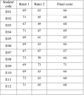
1. The Result of Pre-Test of Experimental Group
The pre-test was conducted on Saturday 10th may 2014. The test meeting
about 1.30 minute at 12.00-13.30 pm in clas x5. They were 36 student who
followed this test. To make it clear, the writer shows the description of pre-test
score of the data achieaved by the experimental group in table 4.1 below:
Table 4.1
The Result of Pre Test Score of Experimental Group
Student'
code Rater 1 Rater 2 Final score
E01 69 63 66
E02 71 65 68
E03 67 69 68
E04 71 67 69
E05 69 61 65
E06 69 63 66
E07 67 67 67
E08 73 59 66
E09 69 73 71
E10 69 63 66
E11 73 63 68
Student'
code Rater 1 Rater 2 Final score
E13 69 65 67
E14 67 63 65
E15 67 67 67
E16 71 63 67
E17 69 69 69
E18 71 59 65
E19 75 69 72
E20 69 67 68
E21 67 63 65
E22 75 63 69
E23 67 67 67
E24 73 59 66
E25 75 63 69
E26 69 63 66
E27 71 69 70
E28 75 59 67
E29 69 63 66
E30 73 59 66
E31 69 61 65
E32 75 63 69
E33 73 63 68
E34 69 63 66
E35 73 67 70
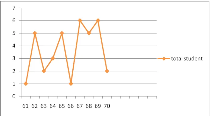
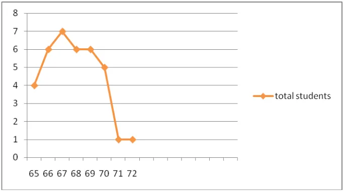
The distribution of students’ pre test scores of experiment group can also
be seen in the following figure.
Figure 4.1 Histogram of Frequency Distribution of Pre Test Scores of Experiment Group
The figure 4.1 showed the pre test scores of students of experiment group.
It can be seen that there was a student got score 61, and 66. There were two
students got score 63, and 70. There were three students got score 64. There were
five students got score 62, 65 and 69. And there were six students got score 67
and 70.
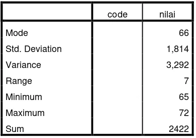
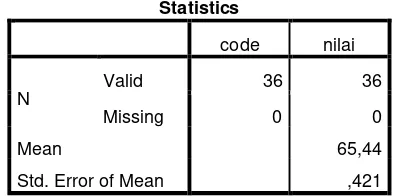
Table 4.2
The Table Calcuation of Mean, Standar Deviation, And Standard Error of Mean of Post Test Score In Control
Group Using Spss 21 Program
Statistics
code nilai
N Valid 36 36
Missing 0 0
Mean 67,28
Std. Error of Mean ,302
code nilai
Mode 66
Std. Deviation 1,814
Variance 3,292
Range 7
Minimum 65
Maximum 72
Sum 2422
2. The Result of Pre Test of Control Group
The pre-test was conducted on Saturday 10th may 2014. The test meeting
about 1.30 minute at 12.00-13.30 pm in clas x5. They were 36 student who
followed this test. To make it clear, the writer shows the description of pre-test
score of the data achieaved by the experimental group in table 4.1 below:
Table 4.3
The result of pre-test score of control group
Student'
code Rater 1 Rater 2 Final score
C01 63 57 60
C02 57 63 60
C03 61 63 62
C04 71 61 66
C05 63 53 58
C06 67 63 65
C07 59 73 66
C08 73 53 63
C09 63 67 65
C10 67 65 66
Student'
code Rater 1 Rater 2 Final score
C12 71 63 67
C13 67 59 63
C14 63 65 64
C15 67 67 67
C16 67 63 65
C17 67 63 65
C18 69 65 67
C19 69 69 69
C20 67 63 65
C21 69 63 66
C22 67 69 68
C23 69 63 66
C24 73 65 69
C25 73 59 66
C26 67 63 65
C27 69 67 68
C28 75 53 64
C29 63 69 66
C30 73 59 66
C31 75 59 67
C32 69 63 66
C33 73 63 68
C34 73 63 68
C35 61 67 64
The distribution of students’ pre test scores of control group can also be
seen in the following figure.
Figure 4.4 Histogram of Frequency Distribution of Pre Test Scores of control Group
The figure 4.4 showed the pre test scores of students of control group. It
can be seen that there was a student got score 58, and 62. There were two students
got score 60, 63, 69,. There were three students got score 64. There were four
students got score 67. There were six student 65 and 68. And there were nine
student got score 66.
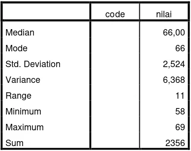
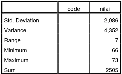
Table 4.5
The Table Calcuation Of Mean, Standar Deviation, And Standard Error of Mean of Pre Test Score In Control Group
Using Spss 21 Program
Statistics
code nilai
N
Valid 36 36
Missing 0 0
Mean 65,44
code nilai
Median 66,00
Mode 66
Std. Deviation 2,524
Variance 6,368
Range 11
Minimum 58
Maximum 69
Sum 2356
3. The Result of Post-Test Experimental Group
The pre-test was conducted on Saturday 31th may 2014. The test meeting
about 1.30 minute at 12.00-13.30 pm in class x5. They were 36 student who
followed this test. To make it clear, the writer shows the description of post-test
score of the data achieved by the experimental group in table 4.1 below:
Table 4.5
The result of post-test score of experimental group
Student'
code Rater 1 Rater 2 Final score
E01 69 73 71
E02 71 63 67
E03 71 69 70
E04 63 69 66
E05 69 67 68
E06 73 69 71
E07 67 73 70
E08 73 65 69
E09 71 75 73
Student'
code Rater 1 Rater 2 Final score
E11 75 69 72
E12 71 69 70
E13 75 59 67
E14 69 67 68
E15 75 69 72
E16 67 69 68
E17 75 65 70
E18 65 67 66
E19 75 71 73
E20 75 69 72
E21 69 71 70
E22 73 69 71
E23 69 69 69
E24 69 65 67
E25 73 65 69
E26 73 71 72
E27 69 73 71
E28 75 59 67
E29 65 67 66
E30 75 67 71
E31 75 65 72
E32 69 71 70
E33 73 71 72
E34 73 69 71
E35 75 65 70
The distribution of students’ post test scores of experimental group can
also be seen in the following figure.
Figure 4.6 Histogram of Frequency Distribution of Post Test Scores of experimental Group
The figure 4.6 showed the post test scores of students of experiment group.
It can be seen that There were two students got score 73. There were three
students got score 66, and 68,. There were four students got score 69. there were
five students got score 67. There were six student got score 71. And there were
eight student got score 70.
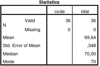
Table 4.7
The Table Calcuation of Mean, Standar Deviation, And Standard Error of Mean of Post Test Score In experimental
Group Using Spss 21 Program
Statistics
code nilai
N
Valid 36 36
Missing 0 0
Mean 69,64
Std. Error of Mean ,348
Median 70,00
code nilai
Std. Deviation 2,086
Variance 4,352
Range 7
Minimum 66
Maximum 73
Sum 2505
4. The Result of Post-Test Control Group
The pre-test was conducted on Saturday 26th may 2014. The test meeting
about 1.30 minute at 12.00-13.30 pm in class x2. They were 36 student who
followed this test. To make it clear, the writer shows the description of post-test
score of the data achieved by the control group below:
Table 4.5
The result of post-test score of cotrol group
Student' code
Rater 1
Rater
2 Final score
C01 69 63 66
C02 71 65 68
C03 67 69 68
C04 71 67 69
C05 69 61 65
C06 69 63 69
C07 67 67 67
C08 73 59 70
C09 69 73 71
C10 69 63 66
Student' code
Rater 1
Rater
2 Final score
C12 71 65 70
C13 69 65 67
C14 67 63 66
C15 67 67 67
C16 71 63 67
C17 69 69 69
C18 71 59 65
C19 75 69 72
C20 69 67 68
C21 67 63 65
C22 75 63 69
C23 67 67 67
C24 73 59 66
C25 75 63 69
C26 69 63 68
C27 71 69 70
C28 75 59 67
C29 69 63 70
C30 73 59 66
C31 69 61 65
C32 75 63 69
C33 73 63 68
C34 69 63 66
C35 73 67 70
The distribution of students’ post test scores of control group can also be
seen in the following figure
The figure 4.1 showed the post test scores of students of control group. It
can be seen that there was a student got score 71, and 72. There were four
students got score 65. There were six students got score , 66, 68 and 69. And there
were seven students got score 67.
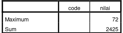
Table 4.7
The Table Calcuation of Mean, Standar Deviation, and Standard Error of Mean of Post Test Score In control Group
Using Spss 21 Program
Statistics
code nilai
N Valid 36 36
Missing 0 0
Mean 67,36
Std. Error of Mean ,304
Median 67,00
Mode 66
Std. Deviation 1,823
Variance 3,323
Range 7
code nilai
Maximum 72
Sum 2425
5. The Comparison of Final Scores Between Experiment Group and Control Group
Based on the data above, it can be seen the comparison in Table
Table 4.8
Control
group
Experiment
Group
66 71
68 67
68 70
69 66
65 68
69 71
67 70
70 69
71 73
66 69
68 72
70 70
67 67
66 68
67 72
67 68
69 70
65 66
72 73
68 72
65 70
69 71
67 69
66 67
69 70
68 72
70 71
67 67
70 66
65 72
69 70
68 72
66 71
70 70
65 67
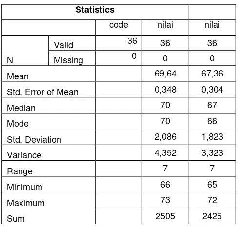
Table 4.9
The Comparison of Final Scores between Control and Experiment Group in Statistic
Statistics
code nilai nilai
N
Valid 36 36 36
Missing 0 0 0
Mean 69,64 67,36
Std. Error of Mean 0,348 0,304
Median 70 67
Mode 70 66
Std. Deviation 2,086 1,823
Variance 4,352 3,323
Range 7 7
Minimum 66 65
Maximum 73 72
Sum 2505 2425
6. Testing Normality and Homogeneity a. Testing normality
One of the requirements in experimental design was the test of normality
assumption. Because of that, the writer used SPSS 21 to measure the normality of
the data. Test Normality of Pre Test and Post Test Scores were described in Table
Tests of Normality
Kolmogorov-Smirnova Shapiro-Wilk
Statistic df Sig. Statistic df Sig.
pretest ,119 72 ,013 ,953 72 ,009
posttest ,125 72 ,007 ,954 72 ,011
a. Lilliefors Significance Correction
Description:
If respondent > 50 used Kolmogorov-Sminornov
If respondent < 50 used Saphiro-Wilk
The criteria of the normality test Pre Test and Post Test is if the value of r
(probability value/critical value) is higher than or equal to the level of significance
alpha defined (r ≥ α = 0.05), it means that, the distribution is normal. Based on the
calculation using SPSS 21 above, the value of r (probably value/critical value)
from Pre test and Post test of the control group and experimental group in
Kolmogorov-Sminornova was higher than level of significance alpha used or r =
0.013> 0.05 (Pre Test) and r = 0.07> 0.05 (Post Test) so that the distributions are
normal. It meant that the students’ scores of in Pre Test and PostTest had a normal
distribution
b. Testing Homogeneity
The definition of Homogeneity of Variance is when all the variables in
statistical data have the same finite or limited variance. When homogeneity of
variance is equal for a statistical model, a simpler computation approach to
analyzing the data can be used due to a low level of uncertainty in the data.
Test of Homogeneity of Variance
Levene Statistic df1 df2 Sig.
posttest Based on Mean 1,068 1 70 ,305
Based on Median ,591 1 70 ,445
Based on Median and with
adjusted df ,591 1 67,852 ,445
Based on trimmed mean 1,027 1 70 ,314
From the table output above can be known that the value of significance
higher than 0.05 so can be concluted that the data have the same variance or
homogene
7. Data Analysis a. Testing hypothesis
The writer applied SPSS 21 program to calculated ttest in testing hypothesis
of the study. The result of the ttest using SPSS 21 program was described in Table
bellow.
Table 4.13
Standard Deviation and Standard Error of X1 and X2 Group Statistics
Group Statistics
code N Mean Std. Deviation Std. Error Mean
score x1 36 77,53 4,205 ,701
Table 4.14
The Calculation ttest Using SPSS 21 Independent Samples Test Independent Samples Test
Levene's
Test for
Equality of
Variances
t-test for Equality of Means
F Sig. t df
Sig. (2-taile d) Mean Difference Std. Error Difference 95% Confidence
Interval of the
Difference
Lower Upper
s c o re Eq u a l v a ri a n c e s a s s u m e d
,717 ,400 4,765 70 ,000 5,417 1,137 3,149 7,684
Eq u a l v a ri a n c e s n o t a s s u m e d
4,765 66,192 ,000 5,417 1,137 3,147 7,686
The table showed the result of ttest calculation using SPSS 21 program.
Since the result of Test test between experimental and control group had
difference scores of variance, it found that the result of tobserved was 4,765.
To examine the truth or false of null hypothesis stating that using
simulation technique does not increase the 10th grade students’ speaking scores,
the result of ttest was interpreted on the result of degree of freedom to get the ttable.
The result of degree of freedom (df) was 70, it found from the total number of
Table 4.15
The Result of tobserved and ttable/ttest Variable tobserved
ttable
Df
5% 1%
X1-X2 4.765 2.000 2.660 70
The interpretation of the result of ttest using SPSS 21 Program, it was found
the tobserved was greater than the ttable at 1% and 5% the level significance or 2.000
< 4.765 > 2.660. It could be interpreted based on the result of calculation that Ha
stating that “the students taught by simulation technique gain better apeaking
performance” was accepted and Ho stating “the students taught by simulation
technique do not gain better speaking achievement” was rejected. It meant that
teaching speaking by using speaking technique increases the 10th grade students’
speaking scores at MAN Model Palangka Raya
b. Manual testing
The writer chose the level of significance in 5%, it mean that the level of
significance of the refusal null hypothesis in 5%. The writer decided the level of
significance at 5% due to the hypothesis type stated on non-directional (two-tailed
test).It meant that the hypothesis cannot directly the prediction of alternative
hypothesis. To test the hypothesis of the study, the writer used t-test statistical
calculation. First, the writer calculated the standard deviation and the standard
error of X1 and X2. It was found the standard deviation and the standard error of
PostTest of X1 and X2 at the previous data presentation. It was described in Table
Table 4.16
Group Statistics
code N Mean Std. Deviation Std. Error Mean
score x1 36 77,53 4,205 ,701
x2 36 72,11 5,371 ,895
TheStandard Deviation and Standard Error of X1 and X2
Description:
X1: Experimental Group
X2: Control Group
The table showed the result of the standard deviation calculation of X1 was
4.205 and the result of the standard error mean calculation was 0.701. The result
of the standard deviation calculation of X2 was 5,371 and the result of the
standard error calculation was 0.895.
The next step, the writer calculated the standard error of the differences mean
between X1 and X2 as follows:
Standard Error of the Difference Mean scores between Variable I and Variable II:
SEM1- SEM2 =
SEM1- SEM2 =
SEM1- SEM2 =
SEM1- SEM2 =
The calculation above showed the standard error of the differences mean
between X1 and X2 was 0.774. Then, it was inserted theto formula to get the value
of tobserved as follows:
to =
to =
to =
to = 4,79646017699115 = 4,796
With the criteria:
If ttest (tobserved) > ttable, Ha is accepted and Ho is rejected.
If ttest (tobserved) < ttable, Ha is rejected and Ho is accepted.
Then, the writer interpreted the result of ttest. Previously, the writer
accounted the degree of freedom (df) with the formula:
Df = (N1 + N2) - 2
= (36 + 36) – 2 = 70
ttable at df 68 at 5% the level of significant = 2,000
The writer chose the level of significance in 5%; it means that the level of
significance of the refusal null hypothesis in 5%. The writer decided the level of
significance at 5% due to the hypothesis typed stated on non-directional
(two-tailed test). It meant that the hypothesis cannot direct the prediction of alternative
hypothesis.
Table 4.17 The Result of ttest
Variable tobserved
ttable
Df
5% 1%
X1-X2 4,765 2,000 2,660 70
Description:
X1 = Experimental Group
X2 = Control Group
tobserved = The Calculated Value
ttable = The Distribution of t value
Df = Degree of Freedom
Based on the result of hypothesis test calculation, it was found that the
value of tobserved was greater than the value of ttable at the level of significance in
5% or 1% that was 2.000 < 4,765 >2.660 It meant Ha was accepted and Ho was
rejected.
It could be interpreted based on the result of calculation that Ha stating
that “the students taught by simulation technique gain better speaking
achievement” was accepted and Ho stating “the students taught by speaking
technique do not gain better speaking achievement” was rejected. It meant that
teaching speaking by using simulation technique increases the 10th grade students’
B. Data Discussion
In this section are discussed under each objective of the study. The writer
have used the data generated by this experiment study as a backdrop in analysing
the benefits and the knowledge that may be gained from using simulation. Does a
learner’s of speaking is improve his/her speaking ability taught by simulation?
That’s thequestion hunting on the writer’s mind. If the hypothesis is true, then the
writer can say that teaching speaking using simulation is accepted, and thus the
later research can be based on this theoretical foundation.
From the data collected after treatment 6 times, the writer found that
students’ speaking scores are listed in twoseparate lines. SPSS version 21 has
been used to perform Pearson Product-moment correlation, which is conducted to
investigate the valididy and realibility of speaking test. The author of this thesis
made two opposite hypotheses (the null and alternative hypotheses), which
needed to be verified by quantitative analysis. From the analysis in 4.15
concluded that the result of the data analysis showed that the simulation technique
gave significance effect on the students’ speaking scores for the 10th
graders of
MAN Model Palangka Raya. The students who were taught using simulation
technique got higher scores than students who were taught without using
simulation technique. It was proved by the mean scores of the students who were
taught using simulation technique was 77.53 and the students who were taught
This is a little bit different to the one of results from previous study by
Nurviana Hardianty: “Improving Speaking Skill Through The Use Of Simulation
Technique” shows that the use of simulation technique is effective in improving
the students’ speaking skill. It can be seen from the result of the data analysis, in
the pre-test the result was 35.4 while in the post-test the result increased to 57.1.
In this case the writer realize that why the writer’ mean score just raise 7 point, it
because there are several extraneous variable inside process collecting the data
such as: (1) the experience of the writer itself is less, (2) the material is boring (3)
non-interesting class room and noisy. But even so the ability of speaking improve
after treatment is true, support by the theory of fee and joys stated that providing
students with guided practice as they develop language skills for meaningful
communication through whole text.
.