Productive efficiency, property rights, and
sustainable renewable resource development
in the mini-purse seine fishery of the Java Sea
INDAH SUSILOWATI
Diponegoro University, Indonesia
NORMAN BARTOO NOAA Fisheries
ISHAK HAJI OMAR Universiti Putra Malaysia
YONGIL JEON
Central Michigan University
K. KUPERAN WorldFish Center
DALE SQUIRES* NOAA Fisheries
NIELS VESTERGAARD University of Southern Denmark
ABSTRACT. The relationship between productive efficiency and sustainable develop-ment of fishing industries in developing countries has received little attention. Ill-structured property rights in common-pool resources lead to a contradiction between private and social technical efficiency, with private and social costs dependent on the level of technical efficiency. Development policies that increase private efficiency can increase the social cost with ill-structured property rights and common-pool resources, and thereby increase social inefficiency. This paper examines this relationship through a case study of the mini purse seine fishery of the Java Sea, and finds that private technical efficiency does not depend on any measurable attributes of human capital, diverges substantially between the peak and off seasons, and differs between vessels more within the off season.
* Corresponding author: Dale Squires, National Marine Fisheries Service, Southwest Fisheries Science Center, 8604 La Jolla Shores Drive, La Jolla, CA 92037, USA. Fax: 858-546-7003. E-mail: [email protected].
1. Introduction
The relationship between productive efficiency and sustainable develop-ment of developing country fisheries has received insufficient attention.1
Harvest rates set at a socially optimal level form a necessary condition for economic growth and development, with steady-state resource stocks at levels at least as high as a target level. Without exclusive use through either fully structured individual property rights or effective regulated common property resource management, however, producers face clear economic incentives to extract from the resource stock at a rate that collectively exceeds the rate required for Pareto-optimal sustainable use (Gordon, 1954; Baland and Platteau, 1996).
The excessive production rate in the open-access, steady-state Nash equilibrium entails not only use of a socially excessive level of inputs, but also the private technical efficiency of production (Squires and Vestergaard, 2001).2 In the stock–flow production technology of natural resource
extraction, higher levels of private technical efficiency increase the output flow for any given level of inputs, state of technology, climatic and other environmental conditions, and abundance, composition, and density of the resource stock. Hence, both the private and external social costs associated with common-pool natural resource extraction, under either open-access or unregulated common property, are dependent not only upon the level of input use but also on the private technical efficiency of production.
In short, a divergence emerges between private and social technical efficiency under ill-structured property rights and ineffective management of regulated common property common-pool resources (Squires and Vestergaard, 2001). Fishers strive to increase their private technical efficiency of production, and hence their exploitation rates, which in turn creates the Pareto-inefficient excessive level of exploitation that collectively follows. A wedge is driven between private and social incentives, whereby individual fishermen or groups have little or no incentive to consider the benefits that accrue to others from the socially optimal exploitation of the common-pool resource stock that accounts for the technological externality
1When we use the term ‘sustainable’, we mean steady-state equilibrium in the resource stock, which arises when the exploitation rate (i.e. catch) equals the growth rate of the resource stock and the biomass of the resource stock remains unchanged. The level of exploitation and the resource stock can be sustainable, but not necessarily at an economic or social optimum. By social optimum, we mean maximum economic yield by which economic rent is maximized. In this regard, sustainable development means some combination of improved economic rent for society and enhanced private profits and incomes for fishers.
arising under ill-formed property rights with a common-pool resource. Poverty and weak private and social institutions – markets, the state, and other bodies of civil society – compound the problem of misaligned private and social institutions under open access or inefficient regulation under common property.
Such a contradiction may exist between private and social technical efficiency in Indonesian commercial fisheries, which are largely unregulated open access. Fisheries development in the past frequently focused upon the harvesting sector and aimed towards resource development through expanded catches and productive efficiency rather than resource management intended to realize sustainable fishing of the resource stock (Priyono and Sumino, 1997). Past fisheries’ development also included the banning of trawlers from inshore fishing grounds (reserving a large share of the grounds and lucrative shrimp for artisanal fishers), zonal restrictions on vessels, expansion of purse seining, and fishery training programs (Sarjono, 1980; Baileyet al., 1987; McElroy, 1991; Bailey, 1997).
Any development policies that increase the private efficiency of production through either increases in technical efficiency, investment, or productivity will tend to increase effective fishing effort and fishing capacity and exacerbate the problems of over-fishing and excess capacity because of the technological resource stock externality due to open-access or unregulated common property. Social welfare losses follow. Policies to increase technical efficiency can operate through captains’ training and extension programs. Investment in fishing gear, engines, and vessels all increase the capital stock in the harvesting sector. Considerable attention has been given to capital formation in the harvesting sector, but heretofore not to the role of technical efficiency in fisheries development other than Squires and Vestergaard (2001).
These capacity-expanding development policies will further reduce the level of the resource stock, unless concomitant policies are introduced to sustainably manage (so that the resource stock level exceeds a minimum target level) the increase in fishing capacity or to correct the ill-structured property rights. Even structuring access to an open-access fishery, such as in Indonesia’s area licensing system (which limits vessels by size in different fishing zones that radiate out from shore), remains an incomplete property right. Vessel numbers are not limited (although the trawl gear is banned). Each individual vessel does not possess an exclusive right, which is fully specified and freely transferable, nor are there well-defined groups in a form of regulated common property. The incomplete property right of limited access does not fully guide incentives to achieve complete internalization of the resource stock externality. The core problem remains that open-access and unregulated common property do not give individuals the proper incentives to harvest in a socially efficient way (Baland and Platteau, 1996).3
This paper begins to address this issue of increasing the private technical efficiency of production, ostensibly to achieve economic growth and lower production costs and the problems it creates for development of Indonesian fisheries that maintain the resource stock above a minimum target level in the face of open-access property rights and the subsequent resource externality. The paper begins to address this issue through a case study of the mini purse seine fishery of the Java Sea. The paper focuses on technical efficiency of these vessels. A full analytical welfare analysis requires a comprehensive bioeconomic model containing technical and allocative efficiency as in Squires and Vestergaard (2001), and an empirical bioeconomic analysis within even a surplus production framework requires cost, revenue, and biological parameters, which are beyond the scope of our data set. Mini purse seine vessels are smaller than the standard purse seine vessels, harvest in coastal waters rather than farther offshore, and primarily target species which include a high proportion of sprat and anchovy (McElroy, 1991).
The paper is organized as follows. The next section, section 2, discusses technical efficiency and resource exploitation when the resource stock is in steady-state equilibrium. Section 3 provides a background to the Java Sea mini purse seine fishery. Section 4 discusses the empirical model – the stochastic production frontier, and the data. Section 5 provides the empirical results. Section 6 offers concluding remarks.
2. Technical efficiency and sustainable resource use
Technical efficiency relative to the ‘best-practice’ production frontier of the vessels in a fishery potentially poses a threat to sustainable resource exploitation at a socially desired target level under open-access or unregulated common property. Output-oriented technical efficiency increases the ‘effective effort’, fishing capacity, catch, and thus the extractive
rate of renewable resources under open access (Kirkley and Squires, 1999).4
Socially excessive extraction rates under open access make it more difficult to achieve sustainable resource use at a target resource stock level and hence sustainable economic development in the fisheries sector.
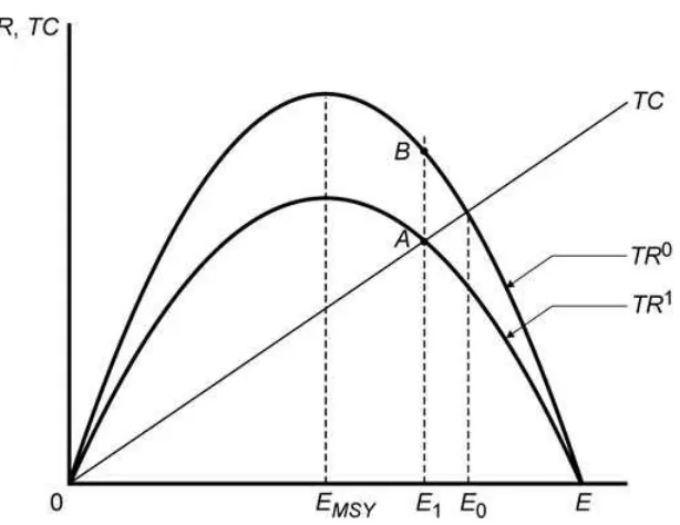
The relationship between output-oriented technical efficiency and sustainable resource use can be illustrated by the well-known Gordon-Schaefer model (Gordon, 1954; Gordon-Schaefer, 1957) in figure 1.5 Let TR
denote total sustainable revenue (i.e. revenue corresponding to a steady-state equilibrium of the resource stock) – the output price is fixed and exogenously determined – TC denote total private cost, and TC = cE, wherecdenotes a constant cost per unit of fishing effort E. When TR= TC, sustainable (steady-state) resource rents,π=TR−TC, are dissipated by excessive fishing effort and the fishery is in an open-access Nash equilibrium in which the resource stock is in steady-state equilibrium. LetTR0denote
total steady-state revenue with full output-oriented technical efficiency, giving an initial Pareto-inefficient Nash equilibrium in open-access with effortE0. SinceE0>EMSYin this example, the resource stock falls below the
maximum sustainable yield (MSY) level, where the MSY resource stock is a sustainable target stock size.
The sustainable total revenue curve is derived from the Schaefer yield– effort curve (Schaefer, 1957). The Schaefer yield–effort curve, in turn, is derived without any explicit assumption about technical efficiency, but the yield–effort curve implicitly assumes full output-oriented technical efficiency (Squires and Vestergaard, 2001). When catch is not harvested
4Output-oriented technical efficiency reflects the ability to obtain maximal output from a given set of inputs. Input-oriented technical efficiency requires the minimum amount of input usage for any given output level (and resource stock in a stock–flow production technology). These measures are equivalent only under constant returns to scale (F¨are and Lovell, 1978). Kumbakhar and Lovell (2000: 44–46) discuss their properties. In addition, estimated technical efficiency for each firm is relative, since it is estimated in terms of distance to a particular best-practice frontier. This frontier is determined by the ‘best-practice’ firms for which no increase in output is feasible holding the input vector, resource stock, environmental conditions, etc. fixed.
The specification of output- or input-oriented technical efficiency is important to the results of this paper (unless there is constant returns to scale, in which case they are equivalent). Under the output-oriented approach, if Indonesian fishers are indeed technically efficient, increasing output by improving resource use would have a negative impact on the resource stock. However, under input-oriented technical efficiency, the output level remains the same and input use becomes more technically efficient, so that additional exploitative pressures are not placed on the resource stock. We select an output-oriented approach because it more closely fits the conditions than an input-oriented approach. With non-malleable physical capital, the capital costs are largely sunk, so that the vessel capital stock is fixed. Moreover, in populous Indonesia, the labor markets are imperfect and the labor force can be characterized by considerable quasi-fixity, another factor contributing to our choice of an output-oriented approach. In addition, the whole issue of excess capacity, of which output-oriented technical efficiency is a major component, generally relies upon an output orientation.
Figure 1.Technical efficiency and the Gordon–Schaefer bioeconomic model.
with full output-oriented technical efficiency, however, sustainable yield, and hence sustainable total revenue, is lower at all levels of effort. The curve TR1in figure 1 depicts the sustainable total revenue when there is not full
output-oriented technical efficiency along with the corresponding Pareto-inefficient Nash equilibrium level of effortE1. Gains in private,
output-oriented technical efficiency to full efficiency raise the measured sustainable total revenue fromTR1to TR0 in figure 1, rent temporarily increases at
the initial level of effortE1 by the amountABin figure 1, and then effort
expands in response fromE1toE0.6A new sustainable, open-access Nash
equilibrium is reached in which all rents are again dissipated, so thatTR0=
TC. This new open-access Nash equilibrium, at an effort level here ofE0>
EMSY, entails a resource stock level below the MSY level and also below the
resource stock level prior to the gains in technical efficiency.
Gains in private technical efficiency may thus pose a social problem under open-access or unregulated common property through the raising of catch rates, increases in ‘effective’ effort and fishing capacity, a new Pareto-inefficient Nash equilibrium, and further reductions in the resource stock (which is socially undesirable if this level is less than a target, such as MSY) (Squires and Vestergaard, 2001). These gains in private technical efficiency raise social costs as the technological resource stock externality is exacerbated. Social costs also increase to the extent that
destructive harvesting practices exacerbate external costs, associated with reduction of the public good formed by ecosystem services, through further degradation of the ecosystem and subsequent loss of resiliency, and reduced environmental carrying capacity. However, under an effective regulatory regime or under an appropriately structured property right (individual or common), gains in private technical efficiency could increase social efficiency and resource rents, if the resource stock lies below the sustainable target level and/or the catch rate lies below the target rate.7
Hence, the social paradox of undesired private technical efficiency gains in fisheries is conditional upon the technological resource stock and ecosystem externalities due to ill-structured property rights. When these property rights are well defined – particularly exclusive use by individuals or well-defined groups with effective self-organization (giving regulated common property), or the regulatory regime maintains capacity near the target level – the social paradox is mitigated in many, albeit not all, instances (Baland and Platteau, 1996). Private and social incentives align and the technological resource stock and ecosystem externalities are internalized by individuals or self-regulating groups.
3. The Java Sea mini purse seine fishery
3.1. Fisheries background
Most Indonesian fishers harvest a number of different species depending on weather conditions and seasonal variability. Medium- and large-scale fishers are able to fish all year round. The waters surrounding Indonesia support a very high level of primary biological productivity, which in turn supports the marine food chain. Currents and winds constantly mix the shallow water column in the Java Sea, especially in coastal waters. River runoff provides nutrients, which contribute to the high natural productivity. The purse seine was introduced to Indonesia and the Java Sea in 1968 at Pekalongan (McElroy, 1991). With the ban on the use of otter trawl gear between 1981 and 1983, purse seine vessels came to dominate medium-scale landings (Baileyet al., 1987; McElroy, 1991). With the trawl ban, the government of Indonesia made credit available to encourage expansion into the pelagic (surface-dwelling) fisheries, particularly purse seining. At that time, pelagic fish stocks were relatively underexploited, especially compared with demersal (bottom-dwelling) fish resources. A number of
trawlers were converted and a number of new purse seine vessels, designed to fish farther offshore, were constructed.
The Java Sea purse seine fleet is based along the north coast of Java. The fleet in Central Java includes both much larger vessels and a coastal fleet – the mini purse seine vessels. With vessel size increasing over time, Central Java was best suited to handle the larger vessels, especially the Nusantara Fish Harbour at Pekalongan and the port of Juwana, followed by the port of Tegal. The number of small coastal landing sites declined with the growth of a few major landing sites. The larger purse seine vessels are powered by diesel engines, whereas a large number of the mini purse seine vessels are powered by longshaft outboard engines (Baileyet al., 1987; McElroy, 1991). The small pelagic fish species, which form the bulk of the purse and mini purse seine catch, show distinct signs of heavy to overexploitation throughout the Java Sea, including those stocks off of north Java (McElroy, 1991). Since 1984, four out of every five tons of finfish caught in the Java Sea have been pelagic species (McElroy, 1991). Total effective fishing effort (measured by days spent at sea per year) has most likely been at a level exceeding maximum sustainable yield since at least 1985, and this measure of effort has continued to increase.8 As the accumulated year classes of
pelagic fish are fished down in previously moderately fished stocks, catches will increasingly depend on the relative strength of just one or two year classes of the main small pelagic fish stocks recruited into the fishery (McElroy, 1991).
The Java Sea small pelagic resource base is heavily exploited throughout its range and for many stocks throughout much of their life cycle by several fishing gears, includingbagan(lift nets), gill nets, and purse seine (McElroy, 1991). Many species are fished sequentially by different gear as they grow and move to deeper, offshore waters (Silvestre and Pauly, 1997). For example, some gear, such asbagan, harvest large proportions of juvenile small pelagic fish, which prevents these fish from reaching full sexual maturity and reproducing (‘recruitment overfishing’) and from growing to a larger size, preventing them from contributing to a larger exploitable biomass (‘growth overfishing’). This ‘recruitment overfishing’, coupled with the high natural mortality, short life spans, and variable recruitment of many small pelagic species, intensifies the expected volatility of stock sizes, catches, and incomes. The sequential fishing by different gears and groups of fishers creates a ‘downstream’ asymmetric resource stock externality, i.e. it introduces a temporal and spatial dimension to the well-known technological resource stock externality.
3.2. Purse seine fishing
Fishing and fish availability are highly seasonal. The severe weather of the monsoon season makes fishing both more difficult and more
dangerous. Heavy rains, rough seas, and strong winds make deploying and retrieving nets more difficult. Transit to and from fishing grounds becomes more difficult. Nutrient levels, currents, bottom conditions, and other environmental factors all combine to affect the availability and abundance of different fish species. Although Indonesia lies well within the tropics, where oceanic primary and secondary biological production does not show strong seasonal fluctuations, the biological production of small pelagic fishes is highly seasonal, being influenced by environmental conditions, most notably by monsoon winds (Pauly and Navaluna, 1983). Organic content, and hence catch rates, decline after the monsoon. During and immediately following monsoon periods, some species of fish may concentrate closer to the shoreline. During periods of calm, which coincide with reduced river discharge, nutrient levels drop and the fish may disperse over a wider area to forage for food. Concentrated fish, especially if the species schools, greatly facilitates the finding and harvesting of fish, whereas fish species that disperse over wider areas and farther from shore are more difficult to find and harvest.
Purse seining has largely superceded the traditional method of seine net fishing of north Java, known aspayang(McElroy, 1991). Unlikepayang, purse seine vessels do not have to maneuver to aim the net at a school of fish. Instead, after locating a shoal (school) of pelagic fish, fishers encircle this shoal by a net. Traditionally, purse seine vessels operate on darker phases of the moon, although there is also an active day fishery. The purse seine net is made of nylon and furnished with floats at the top and a row of heavy brass rings at the bottom through which a rope is reeved (Firth, 1975).
Pelagic species are both migratory and scattered (Bailey et al., 1987). Hence, a fish aggregating device, such as a buoy or bamboo raft with flag pole and trailing coconut leaves or palm fronds, called arumpon, is left in the water in a known fishing area (Firth, 1975; McElroy, 1991). Lamps are generally used at night to attract fish. The vessel stands by, with engine off, until a reasonably sized school accumulates below the aggregating device. The process may be repeated at several rumponsites during the night. Fishing normally ceases or is curtailed over the full moon period when increased ambient light suppresses the phototactic response of small pelagic fishes.
4. Stochastic production frontier
(Sharmaet al., 1999).9The estimation takes the current state of technology,
resource abundance and availability, regulatory structure, and open-access property rights regime as given. The stochastic frontier and technical efficiency results could alter under a different set of conditions.
The translog stochastic production frontier, where symmetry conditions have been imposed, is specified by
lnY =α0+α1lnK +α2lnL+α3lnT+α4lnK2+α5lnL2+α6lnT2
+α7lnKlnL+α8lnKlnT+α9lnLlnT+ǫ (1) Ydenotes total output (catch) in kilograms per trip as the geometric mean of all species landed where revenue shares serve as weights.10The vessel
capital stock (K) is a volumetric measure given by vessel gross registered tons (GRT); labor (L) is the number of crew employed per vessel for a fishing trip, including the captain. The hours per trip (T) serves as a proxy variable for input usage (e.g., diesel and/or gasoline, lubricant and/or oil, ice, and miscellaneous variable inputs).11
The error term, in equation (1) is defined asε=V−U. The two-sided error termVcaptures exogenous stochastic shocks and is assumed to be symmetrical and independently and identically distributed asN(0, σV2). The non-negative error termUcaptures differences in technical inefficiency and is assumed to be an independently distributed non-negative random variable, such thatUis the truncation of a normal distribution at zero, with meanµ=Zδand varianceσU2,N(Zδ,σU2).12The independent distribution of 9The stochastic production frontier’s composite error term includes the one-sided error term, which captures deviations from the best-practice production frontier, and a stochastic error term, which allows for random shocks, measurement error, the combined effects of unspecified input variables in the production frontier, and so forth. The stochastic frontier requires parametric specification of a functional form, the assumption of independence of the two error terms, and a specification for the distributional form of the one-sided error term. The non-parametric method, of which data envelopment analysis (DEA) is the most widely used, has only the one-sided deviation from the best-practice frontier but in the form of an error term. Moreover, the non-parametric approach does not require specification of a particular functional form. However, the deterministic non-para-metric approach does not take into account the possible influence of measurement errors and other noise upon the frontier. Further discussion is provided by Coelli
et al. (1998), Kumbhakar and Lovell (2000), and Ray (2004).
10Other forms of output aggregator functions or output index numbers are possible to aggregate the multiple outputs. For example, revenue shares (which provide approximate measures of transformation elasticities between outputs) can weight the arithmetic mean of outputs, or a translog functional form for the aggregator function could be used to give a Tornqvist index. The form used in this paper, the geometric mean of total output exponentially weighted by revenue shares, gives a discrete approximation to the (continuous) Divisia index and is widely used. 11Both capital and labor are specified as stocks rather than as service flows (which
would be formed by multiplying by hours per trip) to reduce multicollinearity. Due to incomplete responses by survey respondents, only one measure of production time, hours per trip, was available.
VandUallows the separation of statistical noise and technical inefficiency. Z defines a (1×M) vector of explanatory variables associated with the technical inefficiency function, and δ is an (M×1) vector of unknown parameters to be estimated (Battese and Coelli, 1995).13
The technical inefficiency function, comprised of the vector of variables Z, is specified as14
U=δ0+δ1EXP+δ2HOUSEHOLD +δ3CREW +δ4DEDU
+δ5DOFF+δ6DSMALL+W (2)
whereEXPdenotes the captain’s years of fishing experience;HOUSEHOLD denotes total household size (in persons, including the captain);15 and
CREW denotes number of persons per vessel (including captain).16 All
vessels are home-ported in Pekalongan. The three D terms are dummy variables equal to one when: the captain has not received formal education (EDU); the vessel fishes in the off season (OFF);17and the vessel is less than
or equal to 50 GRT (SMALL).
13Kumbhakar et al. (1991) and Reifschneider and Stevenson (1991) first noted the inconsistency between inefficiency effects if in the first stage the error is independently and identically distributed and the predicted inefficiency effects in the second stage are specified as a function of a number of firm-specific factors (which implies that they are not identically distributed unless all the coefficients of the factors are simultaneously equal to zero). The two-stage procedure is unlikely to provide estimates which are as efficient as those that are obtained from the one-step estimation procedure (Coelli, 1996).
14A Huang and Liu (1994) type of model with non-neutral specification of the technical inefficiency model is a possibility. However, there may be correlations between the explanatory variables of the frontier and the inefficiency effects, especially the continuous variables that appear in both equations. In this case, the maximum likelihood (ML) estimators of the parameters would not be consistent. However, the asymptotic properties of the ML estimators for this type of model are currently under investigation (Battese and Broca, 1997, footnotes 1 and 4). 15Household size serves as a proxy variable to capture socio-demographic effects
upon technical inefficiency from family size. Household size, for example, may provide a motivating factor that influences trip length, catch size and composition, choice and number of crew members (some of whom may be included to fulfill familial obligations for example), and the like. Household size is expected to directly relate to technical inefficiency. In addition, while other variables, such as ownership status, age, and schooling experience could be included in the technical inefficiency function, preliminary analysis indicated that their inclusion generated substantial multicollinearity and added little to the model.
16Inclusion of crew size creates a stochastic production frontier that is non-neutral along the lines of Huang and Liu (1994) and Battese and Broca (1997), except that there are no interactions between the inputs of equation (1) and the vectorZof equation (2). The technical inefficiency effects, defined by equation (2), imply that shifts in the frontier for different firms depend, in part, on the levels of the input crew. In addition, we include crew (labor) as a continuous variable, exclude fishing time, and include vessel size as a dummy variable (small vessels) rather than with the same specifications as in equation (1), in order to reduce multicollinearity. 17The peak season includes months 2, 3, 4, i.e. February, March, and April; the
Following the basic approach of Battese and Coelli (1993) and the specification of Kirkleyet al. (1998), the seasonal dummy variable controls for variation in weather and resource availability that varies by season of the year. The vessel has a common production frontier over seasons, since each vessel employs the same production technology and harvests the same resource stock, but technical efficiency is expected to change over seasons. A seasonal dummy variable in the stochastic production frontier would imply discrete shifts in the frontier by season rather than a smooth and continuous best-practice frontier, whereas the same harvesting technology is employed throughout the year. The seasonal dummy variable in the technical inefficiency function allows technical inefficiency to vary by season and allows proper pooling of the balanced panel data over seasons. The interceptδ0 captures the case of a mini purse seine vessel between
50 and 150 GRT; owned and operated by a captain with formal education; and which fishes in the peak season. A random error termWwas added to equation (2) for estimation.
Technical efficiency for each vessel is defined as TE = exp(−U) = exp(−Zδ−W), where exp denotes the exponential operator (Battese and Coelli, 1988). The stochastic frontier, equation (1), and the technical inefficiency function, equation (2), were jointly estimated by maximum likelihood using Frontier 4.1 (Coelli, 1996), under the behavioral hypothesis that fishermen maximize expected profits (Zellneret al., 1966).18
Several hypotheses about the model can be tested by generalized likelihood ratio tests. The first null hypothesis is whether or not technical inefficiency effects are absent, which is specified as: γ=0, where γ = σU2/(σV2+σU2) and lies between 0 and 1. This tests whether or notσU2=0. Non-rejection of the null hypothesis,γ =0, indicates that theUterm should be removed from the model and that the stochastic production frontier is rejected in favor of ordinary least squares estimation (OLS) of the average production function. In this case, the explanatory variables in the technical inefficiency function are included in the production function.19 Given
off season months are 5, 6, 7, 8, i.e. May, June, July, and August; and the stormy season (musim baratan) months are 12 and 1, i.e. December and January.
18The specification of technical inefficiency as unexpected and unknown, or as expected and foreseen, when the firm chooses its inputs affects the specification and estimation of the production function (Kumbhakar, 1987). Given the overwhelming importance of “captain’s skill” in locating and catching fish and the inherent stochastic effects from weather, temperature, and biological variations in fishing, it is likely that technical inefficiency that is unforseen is more important than the foreseen. The point is that technical inefficiency is likely to be never entirely foreseen or unforseen, but in fishing technical inefficiency is more likely to be unexpected and unknown. Thus we specify the technical inefficiency as unexpected or unforseen. Given unknown and unexpected technical inefficiency, the argument of expected profit maximization (Zellneret al., 1966) can be used to treat inputs as exogenous (Kumbhakar, 1987: 336). If technical inefficiency is known to the firm, estimates of the production function parameters obtained directly from the profit function will be inconsistent.
non-rejection of the first null hypothesis, the second null hypothesis is whether or not the functional form of the stochastic production frontier, equation (1), is Cobb–Douglas. The null hypothesis isα4 = α5 = · · · = α9=0 in equation (1). The third hypothesis, tested conditional upon the outcome of the first and second null hypotheses, is whether or not the level of explanatory variables influences the technical inefficiency function, equation (2). Under the assumption that the technical inefficiency effects are distributed as a truncated normal, the null hypothesis is that the matrix of parameters, excluding the intercept termδ0, is null such thatδ1 =δ2= · · · =δ7 =0.20 We begin our testing of the first null hypothesis with the
translog functional form.
4.1. The data
The balanced panel data were collected from the Pekalongan Regency in Central Java from June to July, 1995. Selection of the study areas was arrived at after discussions with the respective local researchers, fisheries officers, and fisher’s association leaders. Susilowati (1998) provides a discussion of the data collection process beyond that presented in this section of the paper.
The following criteria were used in selecting the study area. A multistage sampling method was applied to obtain the sample size of 49 respondents. Fishers were stratified based on gear type and the list of fishing vessels in the area was collected daily from the fisher co-operative unit office for the period of the study in the respective locations. The 49 randomly selected respondents represented 16.3 per cent of the total population of 300 mini purse seine vessels. All of the 49 respondents were from Pekalongan. The sampling unit for this study is the fisher with a decision-making role while at sea. In other words, he is a fishing master. All respondents received their entire income from fishing.
restriction defines a point on the boundary of the parameter space (Coelli, 1996). The critical values are given in table 1 of Kodde and Palm (1986). The number of restrictions, and hence the degrees of freedom for the null hypothesisγ=0, is the difference in the number of parameters in the test of the OLS model versus the stochastic production frontier, equal to one forγ, one forµwith the truncated
normal (associated withδ0, the intercept of the technical inefficiency function) plus the number of terms in the technical inefficiency function, exceptingδ0, which would not enter the traditional mean response function (Battese and Coelli, 1995, footnote 6). In this case, all variables inZ, exceptδ0, would enter the translog production function as log-linear control variables, so that the degrees of freedom forH0:γ=0 is two.
20Not including an intercept parameter (δ
0) in the mean (Zi δ) may result in the
estimators of theδ-parameters, associated with theZ-variables, being biased and the shape of the the distributions of the inefficiency effects,Ui, being unnecessarily
restricted (Battese and Coelli, 1995). Battese and Coelli (1995) note that when theZvector has the value 1 and the coefficients of all other elements ofZare 0, Stevenson’s (1980) model is represented. The intercept δ0 in the technical inefficiency function will have the same interpretation as the µ parameter of
Interviews were carried out by final year students of the Faculty of Economics, Diponegoro University, Indonesia. The interviewers were selected based on the following criteria: working experience as an enumerator, subjects or courses taken in their undergraduate programs, and proficiency in the use of local dialect/language of the respective locations in the study areas. Training was given to all enumerators before they undertook the survey.
Respondents were queried about their ‘typical’ fishing trips in each of three seasons, normal, peak, and off, giving three observations for each respondent, one for each season.21Peak season refers to the season when
catches are usually high (above one standard deviation from the mean catch). Off season refers to the months when catches are low (one standard deviation below the mean) due to the monsoon. Normal season refers to the months when catches are around the mean catch for the year. Oceanographic conditions that vary with monsoons affect surface dwelling and migratory small pelagic fish more than bottom-dwelling demersal fish. Incomplete responses on key variables by all respondents for the normal season required dropping the normal season and its data from the analysis. This left a balanced panel data set of 98 observations, of which 49 were for the peak season and 49 were for the off season.
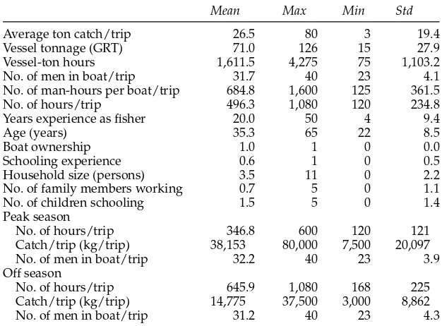
Table 1 reports summary statistics for the Java Sea mini purse seine vessels from a 1995 representative sample, capturing about 16 per cent of the fleet (the data sampling process is described below). The vessels average about 71 gross registered (GRT) with a considerable range from 15 to 126 (table 1). The crew sizes are large, averaging 32 persons with a range of 23 to 40, in keeping with the large crew requirements for hauling in the net. The mini purse seine vessels average about 21 days per trip, although considerable range is found, from a low of around five days to a high of about 45 days. The fishing masters in the fleet are highly experienced, with about 20 years of experience on average, but their formal educational level is comparatively low, where 40 per cent have not received any formal education.
Trip characteristics vary by season (table 1). In the peak season, vessels average a catch per trip of 38,153 kg of fish from a trip of 346.8 hours using 32.2 persons. In the off season, vessels average a catch of 14,775 kg of fish from a trip of 645.9 hours with 31.2 persons onboard. The productivity or catch per hour of the trip declines from the peak to the off season.
5. Empirical results
The translog form of the stochastic production frontier, equation (1), was estimated by maximum likelihood using the trip-level data. The generalized likelihood ratio tests of the three null hypotheses, summarized in table 2, indicate that at the 1 per cent level of significance: (1) the stochastic production frontier is appropriate for the sample of data (H0: γ=0 is
Table 1. Summary statistics of the data for Java Sea mini purse seiners Mean Max Min Std
Average ton catch/trip 26.5 80 3 19.4
Vessel tonnage (GRT) 71.0 126 15 27.9
Vessel-ton hours 1,611.5 4,275 75 1,103.2
No. of men in boat/trip 31.7 40 23 4.1
No. of man-hours per boat/trip 684.8 1,600 125 361.5
No. of hours/trip 496.3 1,080 120 234.8
Years experience as fisher 20.0 50 4 9.4
Age (years) 35.3 65 22 8.5
Boat ownership 1.0 1 0 0.0
Schooling experience 0.6 1 0 0.5
Household size (persons) 3.5 11 0 2.2
No. of family members working 0.7 5 0 1.1
No. of children schooling 1.5 5 0 1.4
Peak season
No. of hours/trip 346.8 600 120 121
Catch/trip (kg/trip) 38,153 80,000 7,500 20,097
No. of men in boat/trip 32.2 40 23 3.9
Off season
No. of hours/trip 645.9 1,080 168 225
Catch/trip (kg/trip) 14,775 37,500 3,000 8,862
No. of men in boat/trip 31.2 40 23 4.3
Notes: GRT=Gross Registered Tons. Schooling experience=0 if no schooling,
=1 if schooling. Boat Ownership=0 if boat owner,=1 otherwise. Socioecono-mic variables pertain to fishing master.
rejected); (2) the Cobb–Douglas functional form is selected for the stochastic production frontier (H0:α4=α5= · · · =α9=0 is not rejected); and (3), the
technical inefficiency function is comprised of the vector of explanatory variables (H0:δ1=δ2= · · · =δ7=0 is rejected).
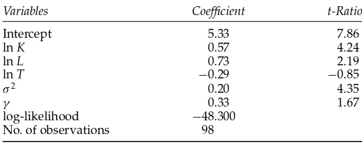
Parameter estimates of the final form of the stochastic production frontier, equation (1), are reported in table 3. The production coefficients for capital (vessel GRT) and labor (number of crew and captain) are statistically significant but the coefficient for time (hours per trip) is not. Hence, although the algebraic sign is negative for time, its statistical insignificance indicates that the production elasticity is zero.22
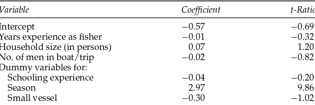
The factors affecting technical inefficiency in the model, given the sample data, can be analyzed by the magnitude, algebraic sign, and significance of the estimated coefficients in equation (2), the technical inefficiency function. Table 4 reports the estimated technical inefficiency function, where the dependent variable is technical inefficiency as opposed to technical efficiency. Thus, a negative sign indicates adecreasein technical inefficiency or anincreasein technical efficiency.
Table 2. Generalized likelihood ratio tests of hypotheses for parameters of the stochastic frontier production function and technical inefficiency function
Likelihood Critical Critical Null hypothesis ratio Df value (5%) value (1%)
1. No stochastic frontier 92.642 2 5.138 8.273
(γ =0)
2. Cobb–Douglas frontier 14.396 6 12.592 16.812
(α5=α7= · · · =α10=0)
3. No technical inefficiency 86.178 6 12.592 16.812
function (δ1=δ2= · · · = δ6=0)
Notes: 1. Test forγ =0 follows mixed chi-square distribution with critical values found in table 1 of Kodde and Palm (1986).
2. Df=degrees of freedom.
3. A truncated-normal distribution is specified for the technical inefficiency error term.
Table 3. Parameter estimates of the stochastic production frontier Variables Coefficient t-Ratio
Intercept 5.33 7.86
lnK 0.57 4.24
lnL 0.73 2.19
lnT −0.29 −0.85
σ2 0.20 4.35
γ 0.33 1.67
log-likelihood −48.300
No. of observations 98
Note: lnK= ln (GRT), lnL= ln (crew), lnT = ln (hours/trip).
The only statistically significant variable in the technical inefficiency function is the dummy variable for the off season, which shows that tech-nical efficiency declines considerably in the off season.23Hence, technical
Table 4. Estimated technical inefficiency function
Variable Coefficient t-Ratio
Intercept −0.57 −0.69
Years experience as fisher −0.01 −0.32
Household size (in persons) 0.07 1.20
No. of men in boat/trip −0.02 −0.82
Dummy variables for:
Schooling experience −0.04 −0.20
Season 2.97 9.86
Small vessel −0.30 −1.02
Notes: 1. Estimated coefficients from a truncated normal distribution for tech-nical inefficiency error term and Cobb–Douglas stochastic production frontier. 2. The definition of the dummy variables are as follows:
Schooling experience dummy=0 if no schooling, and=1 if schooling Season=0 if peak season, and=1 if off season
Small vessel dummy=1 if GRT<40 and 0 otherwise
3. Coefficients obtained from estimation of equation (2), where technical in-efficiency is the dependent variable.
efficiency, which is the most common definition of fishing skill (Kirkley et al., 1998; Squires and Kirkley, 1999), is not related to any of the measurable human capital attributes of the fishing master.24
The distribution of technical efficiency scores, relative to the best practice frontier, is reported in table 5 and depicted in figures 2 and 3. Figure 2 illustrates the technical efficiency scores for each vessel in both the peak and off seasons. In figure 2, the first 49 observations represent the technical efficiency scores in the peak season and the second 49 observations give the scores in the off season. The vessels are ordered the same for both seasons, so that, for example, the first observation corresponds to the same vessel in observation 50. Figure 3 illustrates the technical efficiency scores without distinguishing by season.
The technical efficiency scores combined over both the peak and off seasons range widely, from 0.15 to 0.97 (table 5, figure 3), with a mean score
technical inefficiency across, not simply within, seasons, which requires a pooled model. The inclusion of a random error term, giving the stochastic rather than deterministic frontier, also accounts for the statistical noise. The non-neutral technical inefficiency function approach is attractive, but introduces considerable potential for substantially more multicollinearity in this function, as discussed in footnote 15 above. As discussed in footnote 17, this potential for multicollinearity is why we did not interact crew size with other variables in the technical inefficiency function to give a non-neutral specification.
Table 5. Frequency distribution of technical efficiency scores
Technical efficiency range
[0.0, 0.2) [0.2, 0.4) [0.4, 0.6) [0.6, 0.8) [0.8, 1.0)
Continuous variables 4 42 3 0 49
[count]
1. Years experience as 23.75 20.45 9 0 20.02
fisher [mean]
2. Household size 6.25 3.48 0.33 0 3.51
(persons) [mean]
3. Number of men in 28.5 31.45 30.67 0 32.22
boat/trip [mean] Dummy variables for:
1. School experience No schooling 4 18 0 0 22
Schooling 0 24 3 0 27
2. Season Peak season 0 0 0 0 49
Off season 4 42 3 0 0
3. Small size dummy GRT<40 4 36 1 0 41
Otherwise 0 6 2 0 8
Note: Measures are in terms of efficiency and not inefficiency.
0.0
0.2
0.4
0.6
0.8
1.0
280 290 300 310 320 330 340 350 360 370
fishery id
T
e
c
h
n
ic
a
l
e
ff
ic
ie
n
c
y
Peak season
Off season
0 10 20 30 40 50
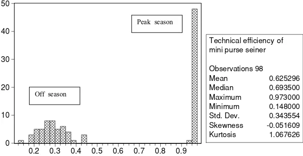
0.2 0.3 0.4 0.5 0.6 0.7 0.8 0.9
Technical efficiency of mini purse seiner
Observations 98
Mean 0.625296 Median 0.693500 Maximum 0.973000 Minimum 0.148000 Std. Dev. 0.343554 Skewness -0.051609 Kurtosis 1.067626 Off season
Peak season
Figure 3. Frequency distribution and summary statistics of technical efficiency by vessel
of 0.625. The mean of 0.625 across all seasons is only slightly lower than those generally found from estimated stochastic production frontiers for developing country agriculture, which is also averaged over all seasons (Ali and Byerlee, 1991; Bravo-Ureta and Pinheiro, 1993, table 1). The mean is also lower than the comparatively high value found by Squireset al. (1998) for the Peninsular Malaysian artisanal gill net fleet. The frequency distribution over all seasons (figure 3) sharply contrasts with that typically found in developing country agriculture over all seasons, where the agricultural distribution is typically skewed toward higher efficiency levels. In sum, the vast majority of the Java Sea mini purse seine vessels have either high or low efficiency levels over the off and peak seasons of the year, respectively, and the low efficiency group faces substantial scope for technical efficiency gains, given the state of their technology and resource abundance.
technical efficiency scores is much lower in the peak season than in the off season. The technical efficiency score of all but four vessels in the off season ranges from 0.20 to 0.40, with four vessels below 0.20 (table 5). During the peak season, all vessels fall in the 0.80 to 1.0 range (table 5).
Most fishers apparently harvest close to the best-practice frontier in the peak season, when conditions are most favorable. Only during the off season, when conditions are least favorable, do substantial inter-vessel differences in technical efficiency appear. Interpreting technical efficiency as fishing skill (Kirkleyet al., 1998; Squires and Kirkley, 1999), it is apparent that the most skilled skippers respond best to the less favorable fishing conditions by maintaining comparatively high catch levels, given their input bundle, while less skilled skippers respond with much less success.
Resource abundance and especially availability fall off during the off season. Stormy weather and rough seas make sailing, locating fish, and on-deck operations more difficult. The number of hours per trip about doubles and mean catch per trip more than halves compared with the peak season, although the number of men in the boat falls by one. Hence, the immediate source of efficiency decline in the monsoon season is clear: a much lower volume of fish is caught during a much lengthier fishing trip. The greater difficulty in following the migratory paths of fish and finding the fish may also contribute. These immediate factors in turn are the consequence of reduced resource availability and less favorable operating conditions.
Campbell and Hand (1998) also found statistically significant seasonal variation in technical inefficiency in the Solomon Islands pole-and-line fishery. Similar to the results in the Java Sea mini purse seine fishery, all Solomon Island vessels tended to perform reasonably well in the good season. However, only the more efficient vessels tended to maintain catch rates and efficiency when stock abundance or availability was low and fishing conditions became less favorable.
6. Concluding remarks
Three key points emerge from the empirical analysis of technical efficiency in the mini purse seine fleet of the Java Sea. First, private technical efficiency, and hence fishing skill, does not depend on any measurable attributes of human capital or on readily available socio-demographic variables of the fishing master. In contrast, measurable attributes of the farmer’s human capital, such as education, are often found significant in studies of technical efficiency in developing country agriculture (Ali and Byerlee, 1991; Bravo-Ureta and Pinheiro, 1993). In agricultural development, these attributes give public policy a handle by which to improve or control efficiency, but no such readily observable handle exists for this fishery. Second, technical efficiency in this fishery varies substantially between seasons, with a sharp drop during the monsoon season, and in the peak season scores for technical efficiency of individual vessels scores are comparatively high. Third, there is little variation in each vessel’s technical efficiency scores during the peak season, but increased variation during the off season.
empirical findings suggest that, in this fishery, however, attempts to manage private technical efficiency through training programs and extension may be largely ineffective because of the paradox between private and social technical efficiency under ill-structured property rights.
The minimal variation in technical efficiency among vessels and the overall high level of technical efficiency during the peak season indicate that the sustainable yield and total revenue curve during the peak season closely correspond to those denoted TR0 in figure 1 and that the effort
level corresponding toE1lies very close toE0and, in addition, ‘effective’
effort lies very close to ‘nominal’ effort. The situation differs during the off season, but it is unclear how a development policy could raise the level of technical efficiency, given the empirical results, so that the short-run gapABin figure 1 and the gap between ‘effective’ and ‘nominal’ effort are both likely to persist in the off season. In sum, for this fishery, the issue of technical efficiency does not appear to pose a threat to sustainable resource exploitation and hence sustainable development. In fact, the low level of technical efficiency in the off season serves to help conserve the resource stock from excessive exploitation. The major issue instead is one of the level of input usage and how best to manage it, a topic which extends beyond the limits of this analysis and is left for future research.
References
Aigner, D.J., C.A.K. Lovell, and P. Schmidt (1977), ‘Formulation and estimation of stochastic production function models’,Journal of Econometrics6: 21–37.
Ali, M. and D. Byerlee (1991), ‘Economic efficiency of small farmers in a changing world: a survey of recent evidence’,Journal of International Development3: 1–27. Bailey, C. (1997), ‘Lessons from Indonesia’s trawler ban’,Marine Policy21: 225–235. Bailey, C., A. Dwiponggo, and F. Marahudin (1987), Indonesian Marine Capture
Fisheries, ICLARM Studies and Reviews 10, Manila: International Center for Living Aquatic Resources Management, Jakarta, Indonesia: Directorate General of Fisheries, and Marine Fisheries Research Institute, Ministry of Agriculture, 196 pp.
Baland, J.-M. and J.-P. Platteau (1996),Halting Degradation of Natural Resources: Is There a Role for Rural Communities?Food and Agriculture Organization of the United Nations and Oxford University Press.
Battese, G. and S. Broca (1997), ‘Functional forms of stochastic frontier production functions and models for technical inefficiency effects: a comparative study for wheat farmers in Pakistan’,Journal of Productivity Analysis8: 395–414.
Battese, G. and T. Coelli (1988), ‘Prediction of firm-level technical efficiencies with a generalized frontier production function and panel data’,Journal of Econometrics
38: 387–399.
Battese, G.E. and T.J. Coelli (1993), ‘A stochastic frontier production function incorporating a model for technical inefficiency effects’, Working Papers in Econometrics and Applied Statistics, No. 69, Department of Econometrics, University of New England, Armidale, 22 pp.
Battese, G.E. and T.J. Coelli (1995), ‘A model for technical inefficiency for panel data’,
Empirical Economics20: 325–332.
Campbell, H.F. and A.J. Hand (1998), ‘Joint ventures and technology transfer: the Solomon Islands pole-and-line fishery’,Journal of Development Economics57: 421– 442.
Coelli, T. (1995), ‘Recent developments in frontier modelling and efficiency measurement’,Australian Journal of Agricultural Economics39: 219–245.
Coelli, T. (1996), ‘A guide to Frontier 4.1: a computer program for stochastic production and cost function estimation’, Department of Econometrics, University of New England, Armidale, Australia.
Coelli, T., D.S.P. Rao, and G.E. Battese (1998), An Introduction to Efficiency and Productive Analysis, Dordrecht: Kluwer Academic Publishers.
F¨are, R. and C.A.K. Lovell (1978), ‘Measuring the technical efficiency of production’,
Journal of Economic Theory19: 150–162.
Firth, R. (1975),Malay Fishermen: Their Peasant Economy, 2nd edn, New York: Norton. Food and Agriculture Organization (FAO) (1983), Expert consultation on the regu-lation of fishing effort (fishing mortality)’, FAO Fisheries Report No. 289, Rome. Gordon, H. (1954), ‘The economic theory of a common-property resource: the
fishery’,Journal of Political Economy62: 124–142.
Hannesson, R. (1983), ‘Bioeconomic production function in fisheries: theoretical and empirical analysis’,Canadian Journal of Fisheries and Aquatic Sciences40: 968–982. Homans, F. and J. Wilen, (1997), ‘A model of regulated open access resource use’,
Journal of Environmental Economics and Management32: 1–21.
Huang, C.J. and J.T. Liu (1994), ‘Estimation of a non-neutral stochastic frontier production function’,Journal of Productivity Analysis52: 171–180.
Jondrow, J., C.A.K. Lovell, I. Materov, and P. Schmidt (1982), ‘On the estimation of technical inefficiency in the stochastic frontier production function model’,Journal of Econometrics19: 239–285.
Kirkley, J., D. Squires, and I. Strand, Jr (1995), ‘Assessing technical efficiency in commercial fisheries: the Mid-Atlantic sea scallop fishery’, American Journal of Agricultural Economics77: 686–697.
Kirkley, J., D. Squires, and I. Strand, Jr (1998), ‘Characterizing managerial skill and technical efficiency in a fishery’,Journal of Productivity Analysis9: 145–160. Kirkley, J. and D. Squires (1999), ‘Measuring capacity and capacity utilization in
fisheries’, in D. Greboval (ed.), Managing Fishing Capacity: Selected Papers on Underlying Concepts and Issues, FAO Fisheries Technical Paper No. 386, Food and Agriculture Organization of the United Nations, Rome.
Kodde, D. and F. Palm (1986), ‘Wald criteria for jointly testing equality and inequality restrictions’,Econometrica54: 1243–1248.
Kumbhakar, S. (1987), ‘The specification of technical and allocative inefficiency in stochastic production and profit frontiers’,Journal of Econometrics34: 335–348. Kumbhakar, S., S.C. Ghosh, and J.T. McGuckin (1991), ‘A generalised production
frontier approach for estimating determinants of inefficiency in US dairy farms’,
Journal of Business and Economic Statistics9: 279–286.
Kumbhakar, S.C. and C.A.K. Lovell (2000),Stochastic Frontier Analysis, Cambridge: Cambridge University Press.
Martosubroto, P. (1996), ‘Structure and dynamics of the demersal resources of the Java Sea, 1975–1979’, in G. Silvestre and D. Pauly (eds), Status and Management of Tropical Coastal Fisheries in Asia, Manila: Asian Development Bank and International Center for Living Aquatic Resources Management, pp. 62–76. McElroy, J. (1991), ‘The Java Sea purse seine fishery: a modern-day “Tragedy of the
Commons”?’,Marine Policy15: 255–271.
Pauly, D. and N. Navaluna (1983), ‘Monsoon-induced seasonality in the recruitment of Philippine fishes’, in G. Sharp and J. Csirke (eds),Proceedings of the Expert Consultation to Examine Changes in Abundance and Species Composition of Neritic Fish Resources, FAO Fisheries Report3: 823–833.
Priyono, B. and Sumiono, B. (1997), ‘The marine fisheries of Indonesia, with emphasis on the coastal demersal stocks of the Sunda Shelf’, in G. Silvestre and D. Pauly (eds), Status and Management of Tropical Coastal Fisheries in Asia, Manila: Asian Development Bank and International Center for Living Aquatic Resources Management, pp. 38–46.
Ray, S. (2004),Data Envelopment Analysis: Theory and Techniques for Economics and Operations Research, Cambridge: Cambridge University Press.
Reifschneider, D. and R. Stevenson (1991), ‘Systematic departures from the frontier: a framework for the analysis of firm efficiency’,International Economic Review32: 715–723.
Sarjono, I. (1980), ‘Trawlers banned in Indonesia’,ICLARM Newsletter3: 3.
Schaefer, M. (1957), ‘Some considerations of population dynamics and economics in relation to the management of marine fisheries’,Journal of the Fisheries Research Board of Canada14: 669–681.
Sharma, K.R. and P.S. Leung (1999), ‘Technical efficiency of the longline fishery in Hawaii: an application of stochastic production frontier’, Marine Resource Economics13: 259–274.
Sharma, K.R., Leung, P.S., and H.M. Zaleski (1999), ‘Technical, allocative and economic efficiencies in swine production in Hawaii: a comparison of parametric and nonparametric approaches’,Agricultural Economics20, 20–35.
Silvestre, G. and D. Pauly (1997), ‘Management of tropical coastal fisheries in Asia: an overview of key challenges and opportunities’, in G. Silvestre and D. Pauly (eds),Status and Management of Tropical Coastal Fisheries in Asia, Manila: Asian Development Bank and International Center for Living Aquatic Resources Management, pp. 8–25.
Squires, D., Q. Grafton, F. Alam, and O. Ishak (1998), ‘Where the land meets the sea: integrated sustainable fisheries development and artisanal fishing’, Discussion Paper No. 98-26, Department of Economics, University of California, San Diego. Squires, D. and J. Kirkley (1999), ‘Skipper skill and panel data in fishing industries’,
Canadian Journal of Fisheries and Aquatic Sciences56: 2011–2018.
Squires, D. and N. Vestergaard, (2001), ‘The paradox of private efficiency and social inefficiency with common-pool resources’, Mimeo, Southwest Fisheries Science Center, La Jolla, CA. (Revised 2003, University of Southern Denmark).
Stevenson, R.E. (1980), ‘Likelihood functions for generalized stochastic frontier estimation’,Journal of Econometrics13: 343–366.
Susilowati, I. (1998), ‘Economics of regulatory compliance in fisheries of Indonesia, Malaysia, and the Philippines’, Unpublished Ph.D. dissertation, Universiti Putra Malaysia.
Wilen, J. (1988), ‘Limited entry licensing: a retrospective assessment’,Marine Resource Economics5: 313–324.