Numerical Methods of Exploration Seismology

(1)

Numerical Methods

of

Exploration Seismology

with algorithms in MATLAB

Gary F. Margrave

Department of Geology and Geophysics

The University of Calgary

(2)

Preface

The most important thing to know about this draft is that it is unﬁnished. This means that it must be expected to have rough passages, incomplete sections, missing references, and references to nonexistent material. Despite these shortcomings, I hope this document will be welcomed for its description of the CREWES MATLAB software and its discussion of velocity, raytracing and migration algorithms. I only ask that the reader be tolerant of the rough state of these notes. Suggestions for the improvement of the present material or for the inclusion of other subjects are most welcome.

Exploration seismology is a complex technology that blends advanced physics, mathematics and computation. Often, the computational aspect is neglected in teaching because, traditionally, seismic processing software is part of an expensive and complex system. In contrast, this book is structured around a set of computer algorithms that run eﬀectively on a small personal computer. These algorithms are written in MATLAB code and so the reader should ﬁnd access to a MATLAB installation. This is not the roadblock that it might seem because MATLAB is rapidly gaining popularity and the student version costs little more than a typical textbook.

The algorithms are grouped into a small number oftoolboxesthat eﬀectively extend the function-ality of MATLAB. This allows the student to experiment with the algorithms as part of the process of study. For those who only wish to gain a conceptual overview of the subject, this may not be an advantage and they should probably seek a more appropriate book. On the other hand, those who wish to master the subject and perhaps extend it through the development of new methods, are my intended audience. The study of these algorithms, including running them on actual data, greatly enriches learning.

The writing of this book has been on my mind for many years though it has only become physical relatively recently. The material is the accumulation of many years of experience in both the hydro-carbon exploration industry and the academic world. The subject matter encompasses the breadth of exploration seismology but, in detail, reﬂects my personal biases. In this preliminary edition, the subject matter includes raytracing, elementary migration, some aspects of wave-equation mod-elling, and velocity manipulation. Eventually, it will also include theoretical seismograms, wavelets, amplitude adjustment, deconvolution, ﬁltering (1D and 2D), statics adjustment, normal moveout removal, stacking and more. Most of the codes for these purposes already exists and have been used in research and teaching at the University of Calgary since 1995.

During the past year, Larry Lines and Sven Treitel have been a constant source of encouragement and assistance. Pat Daley’s guidance with the raytracing algorithms has been most helpful. Pat, Larry, Sven, Dave Henley, and Peter Manning have graciously served as editors and test readers. Many students and staﬀ with CREWES have stress-tested the MATLAB codes. Henry Bland’s technical computer support has been essential. Rob Stewart and Don Lawton have been there with moral support on many occasions.

I thank you for taking the time to examine this document and I hope that you ﬁnd it rewarding.

(3)

Chapter 1

Introduction

1.1

Scope and Prerequisites

This is a book about a complex and diverse subject: the numerical algorithms used to process exploration seismic data to produce images of the earth’s crust. The techniques involved range from simple and graphical to complex and numerical. More often than not, they tend towards the latter. The methods frequently use advanced concepts from physics, mathematics, numerical analysis, and computation. This requires the reader to have a background in these subjects at approximately the level of an advanced undergraduate or beginning graduate student in geophysics or physics. This need not include experience in exploration seismology but such would be helpful.

Seismic datasets are often very large and have historically strained computer storage capacities. This, along with the complexity of the underlying physics, has also strongly challenged computation throughput. These diﬃculties have been a signiﬁcant stimulus to the development of computing technology. In 1980, a 3D migration1 _{was only possible in the advanced computing centers of}

the largest oil companies. At that time, a 50,000 trace 3D dataset would take weeks to migrate on a dedicated, multi-million dollar, computer system. Today, much larger datasets are routinely migrated by companies and individuals around the world, often on computers costing less than $5000. The eﬀective use of this book, including working the computer exercises, requires access to a signiﬁcant machine (at least a late-model PC or Macintosh) with MATLAB installed and having more than 64 mb of RAM and 10 gb of disk.

Though numerical algorithms, coded in MATLAB, will be found throughout this book, this is not a book primarily about MATLAB. It is quite feasible for the reader to plan to learn MATLAB concurrently with working through this book, but a separate reference work on MATLAB is highly recommended. In addition to the reference works published by The MathWorks (the makers of MATLAB), there are many excellent, independent guides in print such as Etter (1996), Hanselman and Littleﬁeld (1998), Redfern and Campbell (1998) and the very recent Higham and Higham (2000). In addition, the student edition of MATLAB is a bargain and comes with a very good reference manual. If you already own a MATLAB reference, then stick with it until it proves inadequate. The website of The MathWorks is worth a visit because it contains an extensive database of books about MATLAB.

Though this book does not teach MATLAB at an introductory level, it illustrates a variety of advanced techniques designed to maximize the eﬃciency of working with large datasets. As

1

Migrationrefers to the fundamental step in creating an earth image from scattered data.

(6)

with many MATLAB applications, it helps greatly if the reader has had some experience with linear algebra. Hopefully, the concepts of matrix, row vector, column vector, and systems of linear equations will be familiar.

1.1.1

Why MATLAB?

A few remarks are appropriate concerning the choice of the MATLAB language as a vehicle for presenting numerical algorithms. Why not choose a more traditional language like C or Fortran, or an object oriented language like C++ or Java?

MATLAB was not available until the latter part of the 1980’s, and prior to that, Fortran was the language of choice for scientiﬁc computations. Though C was also a possibility, its lack of a built-in facility for complex numbers was a considerable drawback. On the other hand, Fortran lacked some of C’s advantages such as structures, pointers, and dynamic memory allocation.

The appearance of MATLAB changed the face of scientific computing for many practitioners, this author included. MATLAB evolved from the Linpack package that was familiar to Fortran programmers as a robust collection of tools for linear algebra. However, MATLAB also introduced a new vector-oriented programming language, an interactive environment, and built-in graphics. These features offered sufficient advantages that users found their productivity was significantly increased over the more traditional environments. Since then, MATLAB has evolved to have a large array of numerical tools, both commercial and shareware, excellent 2D and 3D graphics, object-oriented extensions, and a built-in interactive debugger.

Of course, C and Fortran have evolved as well. C has led to C++ and Fortran to Fortran90. Though both of these languages have their adherents, neither seems to oﬀer as complete a package as does MATLAB. For example, the inclusion of a graphics facility in the language itself is a major boon. It means that MATLAB programs that use graphics are standard throughout the world and run the same on all supported platforms. It also leads to the ability to graphically display data arrays at a breakpoint in the debugger. These are useful practical advantages especially when working with large datasets.

The vector syntax of MATLAB once mastered, leads to more concise code than most other languages. Setting one matrix equal to the transpose of another through a statement like A=B’;is much more transparent than something like

do i=1,n do j=1,m

A(i,j)=B(j,i) enddo

enddo

Also, for the beginner, it is actually easier to learn the vector approach that does not require so many explicit loops. For someone well-versed in Fortran, it can be diﬃcult to un-learn this habit, but it is well worth the eﬀort.

(7)

1.2. MATLAB CONVENTIONS USED IN THIS BOOK 3

Traditional languages like C and Fortran originated in an era when computers were room-sized behemoths and resources were scarce. As a result, these languages are oriented towards simplifying the task of the computer at the expense of the human programmer. Their cryptic syntax leads to eﬃciencies in memory allocation and computation speed that were essential at the time. However, times have changed and computers are relatively plentiful, powerful, and cheap. It now makes sense to shift more of the burden to the computer to free the human to work at a higher level. Spending an extra $100 to buy more RAM may be more sensible than developing a complex data handling scheme to ﬁt a problem into less space. In this sense, MATLAB is a higher-level language that frees the programmer from technical details to allow time to concentrate on the real problem.

Of course, there are always people who see these choices diﬀerently. Those in disagreement with the reasons cited here for MATLAB can perhaps take some comfort in the fact that MATLAB syntax is fairly similar to C or Fortran and translation is not diﬃcult. Also, The MathWorks markets a MATLAB ”compiler” that emits C code that can be run through a C compiler.

1.1.2

Legal matters

It will not take long to discover that the MATLAB source code files supplied with this book all have a legal contract within them. Please take time to read it at least once. The essence of the contract is that you are free to use this code for non-profit education or research but otherwise must purchase a commercial license from the author. Explicitly, if you are a student at a University (or other school) or work for a University or other non-profit organization, then don’t worry just have fun. If you work for a commercial company and wish to use this code in any work that has the potential of profit, then you must purchase a license. If you are employed by a commercial company, then you may use this code on your own time for self-education, but any use of it on company time requires a license. If your company is a corporate sponsor of CREWES (The Consortium for Research in Elastic Wave Exploration Seismology at the University of Calgary) then you automatically have a license. Under no circumstances may you resell this code or any part of it. By using the code, you are agreeing to these terms.

1.2

MATLAB conventions used in this book

There are literally hundreds of MATLABfunctions that accompany this book (and hundreds more that come with MATLAB). Since this is not a book about MATLAB, most of these functions will not be examined in any detail. However, all have full online documentation, and their code is liberally sprinkled with comments. It is hoped that this book will provide the foundation necessary to enable the user to use and understand all of these commands at whatever level necessary.

Typographic style variations are employed here to convey additional information about MATLAB functions. A function name presented like plot refers to a MATLAB function supplied by The MathWorks as part of the standard MATLAB package. A function name presented like dbspec refers to a function provided with this book. Moreover, the name NumMethToolbox refers to the entire collection of software provided in this book.

MATLAB code will be presented in small numbered packages titled Code Snippet. An example is the code required to convert an amplitude spectrum from linear to decibel scale:

Code Snippet 1.2.1. This code computes a wavelet and its amplitude spectrum on both linear and decibel scales. It makes Figure 1.1.

(8)

0 0.02 0.04 0.06 0.08 0.1 0.12 0.14 0.16 0.18 0.2 −0.1

−0.05 0 0.05 0.1

time (sec)

0 50 100 150 200 250

0 0.5 1

Hz

linear scale

0 50 100 150 200 250

−60 −40 −20 0

Hz

dd down

Figure 1.1: A minimum phase wavelet (top), its amplitude spec-trum plotted on a linear scale (middle), and its amplitude specspec-trum plotted with a decibel scale (bottom).

3 _{Amp=abs(Wavem);}

4 _{dbAmp=20*log10(Amp/max(Amp));}

5 _{subplot(3,1,1);plot(t,wavem);xlabel(’time (sec)’)}

6 _{subplot(3,1,2);plot(f,abs(Amp));xlabel(’Hz’);ylabel(’linear scale’)} 7 _{subplot(3,1,3);plot(f,dbAmp);xlabel(’Hz’);ylabel(’db down’)}

End Code

The actual MATLAB code is displayed in an upright typewriter font while introductory remarks are emphasized like this. The Code Snippet does not employ typographic variations to indicate which functions are contained in theNumMethToolbox as is done in the text proper.

It has proven impractical to discuss all of the input parameters for all of the programs shown in Code Snippets. Those germane to the current topic are discussed, but the remainder are left for the reader to explore using MATLAB ’s interactive help facility. For example, in Code Snippet 1.1 wavemin creates a minimum phase wavelet sampled at .002 seconds, with a dominant frequency of 20 Hz, and a length of .2 seconds. Thenfftrl computes the Fourier spectrum of the wavelet and

absconstructs the amplitude spectrum from the complex Fourier spectrum. Finally, the amplitude spectrum is converted to decibels (db) using the formula

Ampdecibels(f) = 20 log

Amp(f) max(Amp(f))

. (1.1)

(9)

1.2. MATLAB CONVENTIONS USED IN THIS BOOK 5

This example illustrates several additional conventions. Seismic traces2 _{are discrete time series}

but the textbook convention of assuming a sample interval of unity in arbitrary units is not appro-priate for practical problems. Instead, two vectors will be used to describe a trace, one to give its amplitude and the other to give the temporal coordinates for the ﬁrst. Thuswavemin returns two vectors (that they are vectors is not obvious from the Code Snippet) withwavem being the wavelet amplitudes andtbeing the time coordinate vector forwavem. Thus the upper part of Figure 1.1 is created by simply cross plotting these two vectors: plot(t,wavem). Similarly, the Fourier spectrum,

Wavem, has a frequency coordinate vector f. Temporal values must always be speciﬁed in seconds and will be returned in seconds and frequency values must always be in Hz. (One Hz is one cycle per second). Milliseconds or radians/second speciﬁcations will never occur in code though both cyclical frequencyf and angular frequencyω may appear in formulae (ω= 2πf).

Seismic traces will always be represented by column vectors whether in the time or Fourier domains. This allows an easy transition to 2-D trace gathers, such as source records and stacked sections, where each trace occupies one column of a matrix. This column vector preference for signals can lead to a class of simple MATLAB errors for the unwary user. For example, suppose a seismic trace s is to be windowed to emphasize its behavior in one zone and de-emphasize it elsewhere. The simplest way to do this is to create a window vectorwin that is the same length assand use MATLAB’s .* (dot-star) operator to multiply each sample on the trace by the corresponding sample of the window. The temptation is to write a code something like this:

Code Snippet 1.2.2. This code creates a synthetic seismogram using the convolutional modelbut then generates an error while trying to apply a (triangular) window.

1 _{[r,t]=reflec(1,.002,.2); %make a synthetic reflectivity} 2 _{[w,tw]=wavemin(.002,20,.2); %make a wavelet}

3 _{s=convm(r,w); % make a synthetic seismic trace}

4 _{n2=round(length(s)/2);}

5 _{win=[linspace(0,1,n2) linspace(1,0,length(s)-n2)]; % a triangular window} 6 _{swin=s.*win; % apply the window to the trace}

End Code

MATLAB’s response to this code is the error message:

??? Error using ==> .* Matrix dimensions must agree. On line 6 ==> swin=s.*win;

The error occurs because thelinspacefunction generates row vectors and sowinis of size 1x501 while s is 501x1. The .* operator requires both operands to be have exactly the same geometry. The simplest ﬁx is to write swin=s.*win(:); which exploits the MATLAB feature that a(:) is reorganized into a column vector (see page 26 for a discussion) regardless of the actual size ofa.

As mentioned previously, two dimensional seismic data gathers will be stored in ordinary matri-ces. Each column is a single trace, and so each row is atime slice. A complete speciﬁcation of such a gather requires both a time coordinate vector,t, and a space coordinate vector,x.

Rarely will the entire code from a function such as wavemin or reflec be presented. This is because the code listings of these functions can span many pages and contain much material that is outside the scope of this book. For example, there are often many lines of code that check input parameters and assign defaults. These tasks have nothing to do with numerical algorithms and so will not be presented or discussed. Of course, the reader is always free to examine the entire codes at leisure.

2

(10)

1.3

Dynamic range and seismic data display

Seismic data tends to be a challenge to computer graphics as well as to computer capacity. A single seismic record can have a tremendous amplitude range. In speaking of this, the termdynamic range is used which refers to a span of real numbers. The range of numerical voltages that a seismic recording system can faithfully handle is called its dynamic range. For example, current digital recording systems use fixed instrument gain and represent amplitudes as a 24 bit integer computer word3_{. The first bit is used to record sign while the last bit tends to fluctuate randomly so effectively}

22 bits are available. This means that the amplitude range can be as large as 222 _≈₁₀6.6_{. Using}

the deﬁnition of a decibel given in equation (1.1), this corresponds to about 132db, an enormous spread of possible values. This 132db range is usually never fully realized when recording signals for a variety of reasons, the most important being the ambient noise levels at the recording site and the instrument gain settings.

In a fixed-gain system, the instrument gain settings are determined to minimize clipping by the analog-to-digital converter while still preserving the smallest possible signal amplitudes. This usually means that some clipping will occur on events nearest the seismic source. A very strong signal should saturate 22-23 bits while a weak signal may only effect the lowest several bits. Thus the precision, which refers to the number of significant digits used to represent a floating point number, steadily declines from the largest to smallest number in the dynamic range.

1.3.1

Single trace plotting and dynamic range

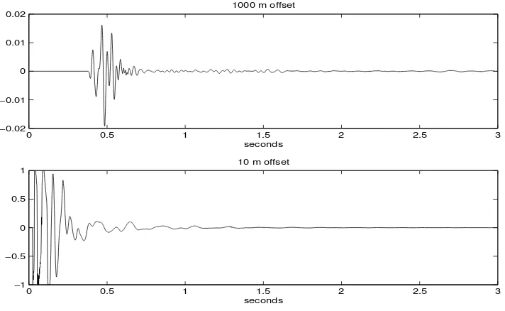
Figure 1.2 was produced with Code Snippet 1.3.1 and shows two real seismic traces recorded in 1997 by CREWES4_{. This type of plot is called a}_{wiggle trace display. The upper trace, called}_tracefar_,

was recorded on the vertical component of a three component geophone placed about 1000 m from the surface location of a dynamite shot. The lower trace, called tracenear, was similar except that it was recorded only 10 m from the shot. (Both traces come from the shot record shown in Figures 1.12 and 1.13.) The dynamite explosion was produced with 4 kg of explosives placed at 18 m depth. Such an explosive charge is about 2 m long so the distance from the top of the charge to the closest geophone was about √162_{+ 10}2 _≈_{19 m while to the farthest geophone was about}

√

162_{+ 1000}2 _≈ _{1000 m. The vertical axes for the two traces indicate the very large amplitude}

diﬀerence between them. If they were plotted on the same axes, tracefarwould appear as a ﬂat horizontal line next to tracenear.

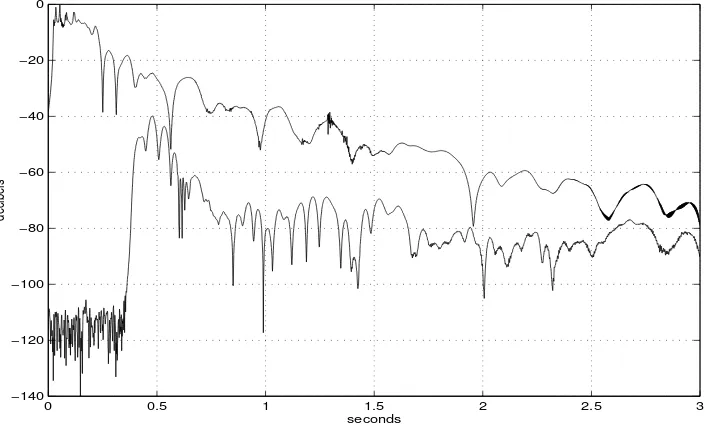
Figure 1.3 (also produced with Code Snippet 1.3.1) shows a more deﬁnitive comparison of the amplitudes of the two traces. Here thetrace envelopes are compared using a decibel scale. A trace envelope is a mathematical estimate of a bounding curve for the signal (this will be investigated more fully later in this book) and is computed usinghilbert, that computes the complex, analytic trace ((Taner et al., 1979) and (Cohen, 1995)), and then takes the absolute value. The conversion to decibels is done with the convenience function todb (for which there is an inverse fromdb). Function todb implements equation (1.1) for both real and complex signals. (In the latter case, todb returns a complex signal whose real part is the amplitude in decibels and whose imaginary part is the phase.) By default, the maximum amplitude for the decibel scale is the maximum absolute value of the signal; but, this may also be speciﬁed as the second input totodb. Function fromdb reconstructs the original signal given the output oftodb.

3

Previous systems used a 16 bit word and variable gain. A four-bit gain word, an 11 bit mantissa, and a sign bit determined the recorded value.

4

(11)

1.3. DYNAMIC RANGE AND SEISMIC DATA DISPLAY 7

0 0.5 1 1.5 2 2.5 3

−0.02 −0.01 0 0.01 0.02

1000 m offset

seconds

0 0.5 1 1.5 2 2.5 3

−1 −0.5 0 0.5 1

10 m offset

seconds

Figure 1.2: (Top) A real seismic trace recorded about 1000 m from a dynamite shot. (Bottom) A similar trace recorded only 10 m from the same shot. See Code Snippet 1.3.1

The close proximity oftracenearto a large explosion produces a very strong ﬁrst arrival while later information (at 3 seconds) has decayed by ∼72 decibels. (To gain familiarity with decibel scales, it is useful to note that 6 db corresponds to a factor of 2. Thus 72 db represents about 72/6

∼12 doublings or a factor of 212_{= 4096.) Alternatively,}_tracefar_{shows peak amplitudes that are}

40db (a factor of 26.7_∼_{100) weaker than}_tracenear_.

Code Snippet 1.3.1. This code loads near and far offset test traces, computes theHilbert envelopes of the traces (with a decibel scale), and produces Figures 1.2 and 1.3.

1 _{clear; load testtrace.mat}

2 _{subplot(2,1,1);plot(t,tracefar);}

3 _{title(’1000 m offset’);xlabel(’seconds’)} 4 _{subplot(2,1,2);plot(t,tracenear);}

5 _{title(’10 m offset’);xlabel(’seconds’)}

6 _{envfar = abs(hilbert(tracefar)); %compute Hilbert envelope} 7 _{envnear = abs(hilbert(tracenear)); %compute Hilbert envelope} 8 _{envdbfar=todb(envfar,max(envnear)); %decibel conversion} 9 _{envdbnear=todb(envnear); %decibel conversion}

10 _figure

11 _{plot(t,[envdbfar envdbnear],’b’);xlabel(’seconds’);ylabel(’decibels’);} 12 _{grid;axis([0 3 -140 0])}

End Code

The first break time is the best estimate of the arrival time of the ﬁrst seismic energy. For

(12)

0 0.5 1 1.5 2 2.5 3 −140

−120 −100 −80 −60 −40 −20 0

seconds

decibels

Figure 1.3: The envelopes of the two traces of Figure 1.2 plotted on a decibel scale. The far oﬀset trace is about 40 db weaker than the near oﬀset and the total dynamic range is about 120 db. See Code Snippet 1.3.1

an indication of ambient noise conditions. That is, it is due to seismic noise caused by wind, traffic, and other effects outside the seismic experiment. Only fortracefaris the first arrival late enough to allow a reasonable sampling of the ambient noise conditions. In this case, the average background noise level is about 120 to 130 db below the peak signals on tracenear. This is very near the expected instrument performance. It is interesting to note that the largest peaks on tracenear

appear to have square tops, indicating clipping, at an amplitude level of 1.0. This occurs because the recording system gain settings were set to just clip the strongest arrivals and therefore distribute the available dynamic range over an amplitude band just beneath these strong arrivals.

Dynamic range is an issue in seismic display as well as recording. It is apparent from Figure 1.2 that either signal fades below visual thresholds at about 1.6 seconds. Checking with the envelopes on Figure 1.3, this suggests that the dynamic range of this display is about 40-50 db. This limitation is controlled by two factors: the total width allotted for the trace plot and the minimum perceivable trace deﬂection. In Figure 1.2 this width is about 1 inch and the minimum discernible wiggle is about .01 inches. Thus the dynamic range is about 10−2 ∼ 40db, in agreement with the earlier visual assessment.

(13)

1.3. DYNAMIC RANGE AND SEISMIC DATA DISPLAY 9

0.2 0.3 0.4 0.5 0.6 0.7 0.8

−0.02 −0.01 0 0.01 0.02 0.03 0.04

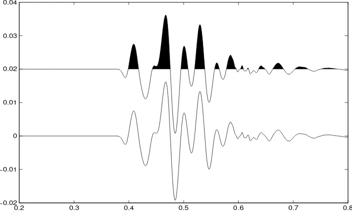
Figure 1.4: A portion of the seismic trace in Figure 1.2 is plotted in WTVA format (top) and WT format (bottom). See Code Snippet 1.3.2

More popular than the wiggle-trace display is the wiggle-trace, variable-area (WTVA) display. Functionwtva (Code Snippet 1.3.2) was be used to create Figure 1.4 where the two display types are contrasted usingtracefar. The WTVA display ﬁlls-in thepeaksof the seismic trace (ortroughs if polarity is reversed) with solid color. Doing this requires determining the zero crossings of the trace which can be expensive if precision is necessary. Function wtva just picks the sample closest to each zero crossing. For more precision, the ﬁnal argument of wtva is a resampling factor which causes the trace to be resampled and then plotted. Also, wtva works like MATLAB ’s low-level

linein that it does not clear the ﬁgure before plotting. This allowswtva to be called repeatedly in a loop to plot a seismic section. The return values ofwtva are MATLAB graphics handles for the “wiggle” and the “variable area” that can be used to further manipulate their graphic properties. (For more information consult your MATLAB reference.) The horizontal line at zero amplitude on the WTVA plot is not usually present in such displays and seems to be a MATLAB graphic artifact.

Code Snippet 1.3.2. The same trace is plotted with wtva andplot. Figure 1.4 is the result.

1 _{clear;load testtrace.mat}

2 _{plot(t,tracefar)}

3 _{[h,hva]=wtva(tracefar+.02,t,’k’,.02,1,-1,1);}

4 _{axis([.2 .8 -.02 .04])}

End Code

(14)

−0.05 0 0.05 0.1 0.15 0.2 0.25 0.3 0.35 0.4 0

0.5

1

1.5

2

2.5

3

6db 12db 18db 24db 30db 36db 42db 48db 54db 60db

seconds

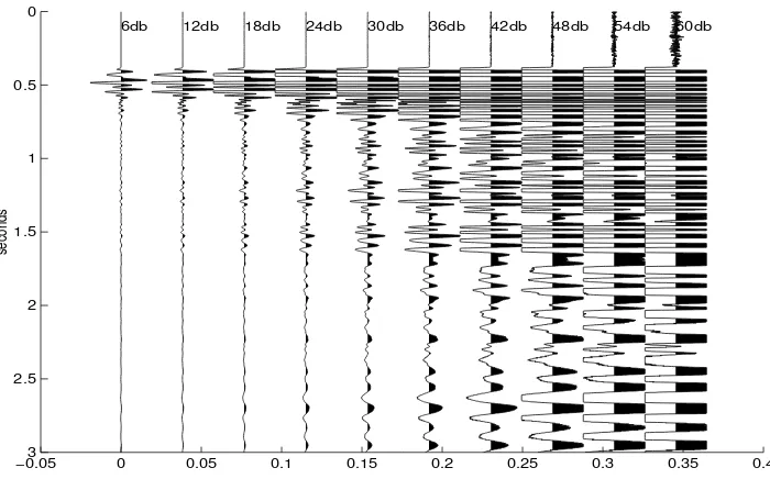
Figure 1.5: The seismic trace in Figure 1.2 is plotted repeatedly with diﬀerent clip levels. The clip levels are annotated on each trace. See Code Snippet 1.3.3

same trace (tracefarat progressively higher clip levels. Functionclip produces the clipped trace that is subsequently rescaled so that the clip level has the same numerical value as the maximum absolute value of the original trace. The eﬀect of clipping is to make the weaker amplitudes more evident at the price of completely distorting the stronger amplitudes. Clipping does not increase the dynamic range, it just shifts the available range to a diﬀerent amplitude band.

Code Snippet 1.3.3. This code makes Figure 1.5. The test trace is plotted repeatedlywith pro-gressivelyhigher clip levels.

1 _{clear;load testtrace.mat} 2 _{amax=max(abs(tracefar));}

3 _{for k=1:10}

4 _{trace_clipped=clip(tracefar,amax*(.5)ˆ(k-1))/((.5)ˆ(k-1));} 5 _{wtva(trace_clipped+(k-1)*2*amax,t,’k’,(k-1)*2*amax,1,1,1);}

6 _{text((k-1)*2*amax,.1,[int2str(k*6) ’db’]);}

7 _end

8 _{flipy;ylabel(’seconds’);}

End Code

Exercise 1.3.1. Use MATLAB to load the test traces shown in Figure 1.2 and displaythem. By appropriatelyzooming your plot, estimate the first break times as accuratelyas you can. What is the approximate velocityof the material between the shot and the geophone? (You mayfind the function

simplezoom useful. After creating your graph, type simplezoom at the MATLAB prompt and then use theleft mouse mutton to draw a zoom box. A double-click will un-zoom.)

(15)

1.3. DYNAMIC RANGE AND SEISMIC DATA DISPLAY 11

0 100 200 300 400 500 600 700 800 900 1000 0

0.1

0.2

0.3

0.4

0.5

0.6

0.7

0.8

0.9

1

seconds

Figure 1.6: A synthetic seismic section plotted in WTVA mode with clipping. See Code Snippet 1.3.4

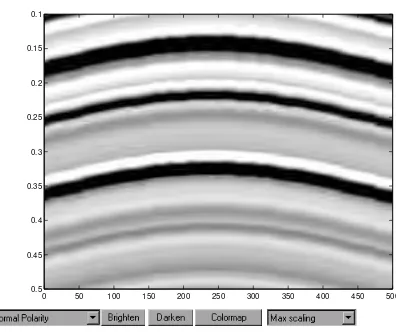
0 50 100 150 200 250 300 350 400 450 500 0.1

0.15

0.2

0.25

0.3

0.35

0.4

0.45

0.5

seconds

Figure 1.7: A zoom (enlargement of a portion) of Figure 1.6. Note the clipping indicated by square-bottomed troughs

Exercise 1.3.3. What is the dynamic range of a seismic wiggle trace display plotted at 10 traces/inch? What about 30 traces/inch?

1.3.2

Multichannel seismic display

Figure 1.5 illustrates the basic idea of a multichannel WTVA display. Assumingntrtraces, the plot width is divided into ntr equal segments to display each trace. A trace is plotted in a given plot segment by adding an appropriate constant to its amplitude. In the general case, these segments may overlap, allowing traces to over-plot one another. After a clip level is chosen, the traces are plotted such that an amplitude equal to the clip level gets atrace excursionto the edges of the trace plot segment. For hardcopy displays, the traces are usually plotted at a speciﬁed number per inch. Figure 1.6 is a synthetic seismic section made by creating a single synthetic seismic trace and then replicating it along a sinusoidal (withx) trajectory. Figure 1.7 is a zoomed portion of the same synthetic seismic section. Functionplotseis made the plot (see Code Snippet 1.3.3), and clipping was intentionally introduced. The square troughs on several events (e.g. near .4 seconds) are the signature of clipping. Functionplotseis provides facilities to control clipping, produce either WT or WTVA displays, change polarity, and more.

Code Snippet 1.3.4. Here we create a simple synthetic seismic section and plot it as a WTVA plot with clipping. Figure 1.6 is the result .

1 _{global NOSIG;NOSIG=1;}

2 _{[r,t]=reflec(1,.002,.2);%make reflectivity}

3 _{nt=length(t);}

4 _{[w,tw]=wavemin(.002,20,.2);%make wavelet} 5 _{s=convm(r,w);%make convolutional seismogram} 6 _{ntr=100;%number of traces}

7 _{seis=zeros(length(s),ntr);%preallocate seismic matrix}

8 _{shift=round(20*(sin([1:ntr]*2*pi/ntr)+1))+1; %a time shift for each trace} 9 _{%load the seismic matrix}

10 _{for k=1:ntr}

(16)

0 100 200 300 400 500 600 700 800 900 0

0.1

0.2

0.3

0.4

0.5

0.6

0.7

0.8

0.9

1

Figure 1.8: A synthetic seismic section plotted as an image using plotimage. Compare with Figure 1.6

0 50 100 150 200 250 300 350 400 450 500 0.1

0.15

0.2

0.25

0.3

0.35

0.4

0.45

0.5

Figure 1.9: A zoom (enlargement of a portion) of Figure 1.8. Compare with Figure 1.7

12 _end

13 _{x=(0:99)*10; %make an x coordinate vector}

14 _{plotseis(seis,t,x,1,5,1,1,’k’);ylabel(’seconds’)}

End Code

Code Snippet 1.3.4 illustrates the use of global variables to control plotting behavior. The global

NOSIG controls the appearance of a signature at the bottom of a ﬁgure created by plotseis. If

NOSIG is set to zero, thenplotseis will annotate the date, time, and user’s name in the bottom right corner of the plot. This is useful in classroom settings when many people are sending nearly identical displays to a shared printer. The user’s name is defined as the value of another global variable, NAME_ (the capitalization and the underscore are important). Display control through global variables is also used in other utilities in the NumMethToolbox(see page 14). An easy way to ensure that these variables are always set as you prefer is to include their definitions in your startup.m file (see your MATLAB reference for further information).

The popularity of the WTVA display has resulted partly because it allows an assessment of the seismic waveform (if unclipped) as it varies along an event of interest. However, because its dynamic range varies inversely with trace spacing it is less suitable for small displays of densely spaced data such as on a computer screen. It also falls short for display of multichannel Fourier spectra where the wiggle shape is not usually desired. For these purposes, image displays are more suitable. In this technique, the display area is divided equally into small rectangles (pixels) and these rectangles are assigned a color (or gray-level) according to the amplitude of the samples within them. On the computer screen, if the number of samples is greater than the number of available pixels, then each pixel represents the average of many samples. Conversely, if the number of pixels exceeds the number of samples, then a single sample can determine the color of many pixels, leading to a blocky appearance.

(17)

1.3. DYNAMIC RANGE AND SEISMIC DATA DISPLAY 13

0 10 20 30 40 50 60 70

0 0.2 0.4 0.6 0.8

1white

black

level number

gray

l

evel

Figure 1.10: A 50% gray curve from seisclrs (center) and its brightened(top) and darkened (bottom) versions.

0 10 20 30 40 50 60 70

0 0.2 0.4 0.6 0.8 1

100 80

60 40

20 white

black

level number

gray

l

evel

Figure 1.11: Various gray level curves from seisclrs for diﬀerentgray pctvalues.

scheme (though these controls are shown in these ﬁgures, in most cases in this book they will be suppressed). The latter item refers to the system by which amplitudes are mapped to gray levels (or colors).

Code Snippet 1.3.5. This example illustrates the behavior of the seisclrs color map. Figures 1.10 and 1.11 are created.

1 _figure;

2 _{global NOBRIGHTEN}

3

4 NOBRIGHTEN=1;

5 _{s=seisclrs(64,50); %make a 50% linear gray ramp} 6 _{sb=brighten(s,.5); %brighten it}

7 _{sd=brighten(s,-.5); %darken it}

8 _{plot(1:64,[s(:,1) sb(:,1) sd(:,1)],’k’)}

9 _{axis([0 70 -.1 1.1])}

10 _{text(1,1.02,’white’);text(50,.02,’black’)} 11 _{xlabel(’level number’);ylabel(’gray_level’);} 12 _{figure; NOBRIGHTEN=0;}

13 _{for k=1:5}

14 _{pct=max([100-(k-1)*20,1]);}

15 _{s=seisclrs(64,pct);}

16 _{line(1:64,s(:,1),’color’,’k’);}

17 _{if(rem(k,2))tt=.1;else;tt=.2;end}

18 _{xt=near(s(:,1),tt);}

19 _{text(xt(1),tt,int2str(pct))}

20 _end

21 _{axis([0 70 -.1 1.1])}

22 _{text(1,1.02,’white’);text(50,-.02,’black’)} 23 _{xlabel(’level number’);ylabel(’gray_level’);}

End Code

(18)

meters

seconds

0 100 200 300 400 500 600 700 800 900 1000 0

0.5

1

1.5

2

2.5

3

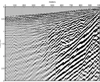
Figure 1.12: A raw shot record displayed using plotimage andmaximum scaling

meters

seconds

0 100 200 300 400 500 600 700 800 900 1000 0

0.5

1

1.5

2

2.5

3

Figure 1.13: The same raw shot record as Figure 1.12 but displayed usingmean scalingwith a clip level (parameter CLIP) of 4.

at level 1 to 0 (black) at level 64. However, this was found to produce overly dark images with little event standout. Instead, seisclrs assigns a certain percentage, calledgray pct, of the 64 levels to the transition from white to black and splits the remaining levels between solid black and solid white. For example, by default this percentage is 50 which means that levels 1 through 16 are solid white, 17 through 48 transition from white to black, and 49 through 64 are solid black. The central curve in Figure 1.10 illustrates this. As a ﬁnal step, seisclrs brightens the curve usingbrighten

to produce the upper curve in Figure 1.10. Figure 1.11 shows the gray scales that result from varying the value ofgray pct.

Given a gray level or color scheme, functionplotimage has two diﬀerent schemes for determining how seismic amplitudes are mapped to the color bins. The simplest method, calledmaximum scaling determines the maximum absolute value in the seismic matrix, assigns this the color black, and the negative of this number is white. All other values map linearly into bins in between. This works well for synthetics, or well-balanced real data, but often disappoints for noisy or raw data because of the data’s very large dynamic range. The alternative, calledmean scaling, measures both the mean, ¯

sand standard deviation σs of the data and assigns the mean to the center of the gray scale. The

ends of the scale are assigned to the values ¯s±CLIPσswhere CLIP is a user-chosen constant. Data

values outside this range are assigned to the ﬁrst or last gray-level bin thereby clipping them. Thus, mean scaling centers the gray scale on the data mean and the extremes of the scale are assigned to a ﬁxed number of standard deviations from the mean. In both of these schemes, neutral gray corresponds to zero (if theseisclrs color map is used).

Figure 1.12 displays a raw shot record using the maximum scaling method with plotimage. (The shot record is contained in the filesmallshot.mat, and the traces used in Figure 1.2 are the first and last trace of this record.) The strong energy near the shot sets the scaling levels and is so much stronger than anything else that most other samples fall into neutral gray in the middle of the scale. On the other hand, figure 1.13 uses mean scaling (and very strong clipping) to show much more of the data character.

(19)

1.3. DYNAMIC RANGE AND SEISMIC DATA DISPLAY 15

seconds

0 100 200 300 400 500 600 700 800 900 0

0.1

0.2

0.3

0.4

0.5

0.6

0.7

0.8

0.9

1

Figure 1.14: A synthetic created to have a 6db decrease with each event displayed by plotimage. See Code Snippet 1.3.7.

0 100 200 300 400 500 600 700 800 900 1000 0

0.1

0.2

0.3

0.4

0.5

0.6

0.7

0.8

0.9

1

seconds

Figure 1.15: The same synthetic as Figure 1.14 displayed withplotseis.

is limited to the setting in which they are deﬁned. For example, a variable calledxdeﬁned in the base workspace (i.e. at the MATLAB prompt≫) can only be referenced by a command issued in the

base workspace. Thus, a function likeplotimage can have its own variablexthat can be changed arbitrarily without aﬀecting the x in the base workspace. In addition, the variables deﬁned in a function are transient, meaning that they are erased after the function ends. Global variables are an exception to these rules. Once declared (either in the base workspace or a function) they remain in existence until explicitly cleared. If, in the base workspace, xis declared to be global, then the

xin plotimage is still independent unlessplotimage also declaresxglobal. Then, both the base workspace andplotimage address the same memory locations forx and changes in one aﬀect the other.

Code Snippet 1.3.6 illustrates the assignment of global variables for plotimage as done in the author’s startup.m ﬁle. These variables only determine the state of a plotimage window at the time it is launched. The user can always manipulate the image as desired using the user interface controls. Any such manipulations will not aﬀect the global variables so that the next plotimage window will launch in exactly the same way.

Code Snippet 1.3.6. This is a portion of the author’s startup.mfile that illustrates the setting of global variables to control plotimage.

1 _{global SCALE_OPT GRAY_PCT NUMBER_OF_COLORS} 2 _{global CLIP COLOR_MAP NOBRIGHTEN NOSIG}

3 SCALE_OPT=2;

4 _{GRAY_PCT=20;}

5 _{NUMBER_OF_COLORS=64;}

6 _CLIP=4;

7 _{COLOR_MAP=’seisclrs’;}

8 _{NOBRIGHTEN=1;}

9 _NOSIG=1;

(20)

Code Snippet 1.3.7. This code creates a synthetic with a 6db decrease for each event and displays it without clipping with both plotimageand plotseis. See Figures 1.14 and 1.15.

1 _{% put an event every 100 ms. Each event decreases in amplitude by 6 db.} 2 _{r=zeros(501,1);dt=.002;ntr=100;}

3 _{t=(0:length(r)-1)*dt;}

4 _amp=1;

5 _{for tk=.1:.1:1;}

6 _{k=round(tk/dt)+1;}

7 _{r(k)=(-1)ˆ(round(tk/.1))*amp;}

8 _amp=amp/2;

9 _end

10 _{w=ricker(.002,60,.1);} 11 _{s=convz(r,w);}

12 _{seis=s*ones(1,ntr);} 13 _{x=10*(0:ntr-1);}

14 _{global SCALE_OPT GRAY_PCT} 15 _{SCALE_OPT=2;GRAY_PCT=100;;}

16 _{plotimage(seis,t,x);ylabel(’seconds’)}

17 _{plotseis(seis,t,x,1,1,1,1,’k’);ylabel(’seconds’)}

End Code

The dynamic range of image and WTVA displays is generally diﬀerent. When both are displayed without clipping using a moderate trace spacing (Figures 1.14 and 1.15), the dynamic range of plotimage (≈30db) tends to be slightly greater than that of plotseis(≈20db). However, the behavior of plotimage is nearly independent of the trace density whileplotseis becomes useless at high densities.

Exercise 1.3.4. Load the file smallshot.mat into your base workspace using the command load and displaythe shot record with plotimage. Studythe online help forplotimageand define the six global variables that control its behavior. Practice changing their values and observe the results. In particular, examine some of the color maps: hsv, hot, cool, gray, bone, copper, pink, white, flag, jet, winter, spring, summer, and autumn. (Be sure to specifythe name of the color map inside single quotes.)

Exercise 1.3.5. Recreate Figures 1.14 and 1.15 using Code Snippet 1.3.7 as a guide. Experiment with different number of traces (ntr) and different program settings to see how dynamic range is affected.

1.3.3

The

plotimage

picking facility

The function plotimage, in addition to displaying seismic data, provides a rudimentary seismic picking facility. This is similar in concept to using MATLAB’s ginput (described in the next section) but is somewhat simpler to use. In concept, this facility simply allows the user to draw any number of straight-line segments (picks) on top the the data display and aﬀords easy access to the coordinates of these picks. The picks can then be used in any subsequent calculation or analysis.

(21)

1.3. DYNAMIC RANGE AND SEISMIC DATA DISPLAY 17

0 100 200 300 400 500 600 700 800 900 1000 0

0.1

0.2

0.3

0.4

0.5

0.6

0.7

0.8

0.9

1

Figure 1.16: This ﬁgure is displayed by Code Snippet 1.3.8 before allowing the user to select points.

0 100 200 300 400 500 600 700 800 900 1000 0

0.1

0.2

0.3

0.4

0.5

0.6

0.7

0.8

0.9

1

Figure 1.17: After the user picks the ﬁrst breaks in Figure 1.16, the picks are drawn on top of the seismic data. See Code Snippet 1.3.8.

for the ﬁrst window will be lost. If desired, this can be avoided by copying the pick list into another variable prior to activating the second picking process.

A pick is made by clicking the left mouse button down at the ﬁrst point of the pick, holding the button down while dragging to the second point, and releasing the button. The pick will be drawn on the screen in a temporary color and then drawn in a permanent color when the mouse is released. The permanent color is controlled by the global variable PICKCOLOR. If this variable has not been set, picks are drawn in red. A single mouse click, made without dragging the mouse and within the bounds of the axes, will delete the most recent pick.

This picking facility is rudimentary in the sense that the picks are established without any numerical calculation involving the data. Furthermore, there is no facility to name a set of picks or to retain their values. Nevertheless, a number of very useful calculations, most notably raytrace migration (see sections 4.2.2 and 4.3.3) are enabled by this. It is also quite feasible to implement a more complete picking facility on this base.

1.3.4

Drawing on top of seismic data

Often it is useful to draw lines or even ﬁlled polygons on top of a seismic data display. This is quite easily done using MATLAB’slineandpatchcommands. Onlylineis discussed here.

Code Snippet 1.3.8 loads the small sample shot record and displays it. The command ginput

halts execution of the script and transfers focus to the current figure. There, the cursor will be changed to a crosshairs and the user is expected to enter a sequence of mouse clicks to define a series of points. In the example shown in Figures 1.16 and 1.17, six points were entered along the first breaks. ginput expects the points to be selected by simple mouse clicks and then the “enter” key is hit to signal completion. The six points are returned as a vector ofxcoordinates,xpick, and a vector oftcoordinates,tpick. Though it is a useful tool,ginputdoes note provide a picking facility such as that described previously. However,ginputworks with any MATLAB graphics display while the picking facility is only available withplotimage.

(22)

coordinates of the nodes of the line to be drawn. If no z coordinates are given, they are assumed zero which causes them to be drawn in the same z plane as the seismic (MATLAB graphics are always 3D even when they appear to be only 2D). Plotting the line atz = 0 usually works but if more mouse clicks are done on the ﬁgure, such as for zooming, then it can happen that the line may get re-drawn ﬁrst with the seismic on top of it. This causes the line to “disappear”. Instead, it is more robust to give the line a vector of z coordinates of unity so that it is guaranteed to always be in front of the seismic.

In addition to (x, y, z) coordinates,lineaccepts an arbitrary length list of (attribute, property) pairs that deﬁne various features of the line. In this case, its color is set tored, its line thickness is set to twice normal, and markers are added to each point. There are many other possible attributes that can be set in this way. To see a list of them, issue the commandget(h)wherehis the handle of a line and MATLAB will display a complete property list. Once the line has been drawn, you can alter any of its properties with thesetcommand. For example,set(h,’color’,’c’) changes the line color to cyan andset(h,’ydata’,get(h,’ydata’)+.1)shifts the line down .1 seconds.

Code Snippet 1.3.8. This example displays the small sample shot record using plotimage and then uses ginput to allow the user to enter points. These points are plotted on top of the seismic data using line. The results are in Figures 1.16 and 1.17.

1 _{load smallshot}

2 _{global SCALE_OPT CLIP}

3 SCALE_OPT=1;CLIP=1;

4 _{plotimage(seis,t,x)}

5 _{axis([0 1000 0 1])}

6 _{[xpick,tpick]=ginput;}

7 _{h=line(xpick,tpick,ones(size(xpick)),’color’,’r’,...}

8 _{’linewidth’,2,’marker’,’*’);}

End Code

1.4

Programming tools

It is recommended that a study course based on this book involve a considerable amount of pro-gramming. Programming in MATLAB has similarities to other languages but it also has its unique quirks. This section discusses some strategies for using MATLAB eﬀectively to explore and manip-ulate seismic datasets. MATLAB has two basic programming constructs,scriptsandfunctions, and program will be used to refer to both.

1.4.1

Scripts

MATLAB is designed to provide a highly interactive environment that allows very rapid testing of ideas. However, unless some care is taken, it is very easy to create results that are nearly irreproducible. This is especially true if a long sequence of complex commands has been entered directly at the MATLAB prompt. A much better approach is to type the commands into a text ﬁle and execute them as a script. This has the virtue that a permanent record is maintained so that the results can be reproduced at any time by simply re-executing the script.

(23)

1.4. PROGRAMMING TOOLS 19

first so-named file in the path, use the which command. Typingwhich foo causes MATLAB to display the complete path to the file that it will execute whenfoois typed.

A good practice is to maintain a folder in MATLAB’s search path that contains the scripts associated with each logically distinct project. These script directories can be managed by creating a further set of control scripts that appropriately manipulate MATLAB’s search path. For example, suppose that most of your MATLAB tools are contained in the directory

C:\Matlab\toolbox\local\mytools

and that you have project scripts stored in

C:\My Documents\project1\scripts

and

C:\My Documents\project2\scripts.

Then, a simple management scheme is to include something like

1 _{global MYPATH}

2 _{if(isempty(MYPATH))}

3 _p=path;

4 _{path([p ’;C:\MatlabR11\toolbox\local\mytools’]);}

5 _MYPATH=path;

6 _else

7 _{path(MYPATH);}

8 _end

in your startup.m ﬁle and then create a script called project1.m that contains

1 _p=path;

2 _{path([p ’;C:\My Documents\project1\scripts’])}

and a similar script for project2. When you launch MATLAB your startup.m establishes your base search path and assigns it to a global variable called MYPATH. Whenever you want to work on project1, you simply typeproject1 and your base path is altered to include the project1 scripts. Typingstartup again restores the base path and typingproject2 sets the path for that project. Of course you could just add all of your projects to your base path but then you cannot have scripts with the same name in each project.

Exercise 1.4.1. Write a script that plots wiggle traces on top of an image plot. Test your script with the synthetic section of Code Snippet 1.3.4. (Hint: plotseisallows its plot to be directed to an existing set of axes instead of creating a new one. The “current” axes can be referred to withgca.)

1.4.2

Functions

The MATLAB function provides a more advanced programming construct than the script. The latter is simply a list of MATLAB commands that execute in the base workspace. Functions execute in their own independent workspace that communicates with the base workspace throughinput and output variables.

The structure of a function

(24)

[output_variable_list]=function_name(input_variable_list).

Rectangular brackets [ . . . ] enclose the list of output variables, while regular parentheses enclose the input variables. Either list can be of any length, and entries are separated by commas. Forclip, there is only one output variable and the [ . . . ] are not required. When the function is invoked, either at the command line or in a program, a choice may be made to supply only the firstninput variables or to accept only the firstmoutput variables. For example, given a function definition like

[x1,x2]=foo(y1,y2), it make be legally invoked with any of

[a,b]=foo(c,d); [a,b]=foo(c); a=foo(c,d); a=foo(c);

The variable names in the function declaration have no relation to those actually used when the function is invoked. For example, whena=foo(c)is issued the variablecbecomes the variable(y1) withinfoo’s workspace and similarly,foo’s x1is returned to become the variable ain the calling workspace. Though it is possible to callfoowithout specifying y2there is no simple way to call it and specifyy2 while omittingy1. Therefore, it is advisable to structure the list of input variables such that the most important ones appear ﬁrst. If an input variable is not supplied, then it must be assigned adefaultvalue by the function.

Code Snippet 1.4.1. A simple MATLAB function to clip a signal.

1 _{function trout=clip(trin,amp);}

2 _{% CLIP performs amplitude clipping on a seismic trace}

3 _%

4 _{% trout=clip(trin,amp)}

5 _%

6 _{% CLIP adjusts only those samples on trin which are greater} 7 _{% in absolute value than ’amp’. These are set equal to amp but} 8 _{% with the sign of the original sample.}

9 _%

10 _{% trin= input trace} 11 _{% amp= clipping amplitude} 12 _{% trout= output trace}

13 _%

14 _{% by G.F. Margrave, May 1991}

15 _%

16 _{if(nargin˜=2)}

17 _{error(’incorrect number of input variables’);}

18 _end

19 _{% find the samples to be clipped} 20 _{indices=find(abs(trin)>amp);}

21 _{% clip them}

22 _trout=trin;

23 _{trout(indices)=sign(trin(indices))*amp;}

End Code

In the example of the functionclip there are two input variables, both mandatory, and one out-put variable. The next few lines after the function definition are all comments (i.e. non-executable) as is indicated by the % sign that precedes each line. The first contiguous block of comments follow-ing the function definition constitutes theonline help. Typinghelp clipat the MATLAB prompt will cause these comment lines to be echoed to your MATLAB window.

(25)

1.4. PROGRAMMING TOOLS 21

directory containing many .m files, causes the first line of each file to be echoed giving a summary of the directory. Next appears one or morefunction prototypes that give examples of correct function calls. After viewing a function’s help file, a prototype can be copied to the command line and edited for the task at hand. The next block of comments gives a longer description of the tasks performed by the function. Then comes a description of each input and output parameter and their defaults, if any. Finally, it is good form to put your name and date at the bottom. If your code is to be used by anyone other than you, this is valuable because it establishes who owns the code and who is responsible for fixes and upgrades.

Following the online help is the body of the code. Lines 16-18 illustrate the use of the auto-matically deﬁned variablenarginthat is equal to the number of input variables supplied at calling. clip requires both input variables so it aborts ifnarginis not two by calling the function error. The assignment ofdefault values for input variables can also be done usingnargin. For example, suppose the ampparameter were to be allowed to default to 1.0. This can be accomplished quite simply with

if(nargin<2) amp=1; end

Lines 20, 22, and 23 actually accomplish the clipping. They illustrate the use of vector addressing and will be discussed more thoroughly in Section 1.5.1.

1.4.3

Coping with errors and the MATLAB debugger

No matter how carefully you work, eventually you will produce code with errors in it. The simplest errors are usually due to mangled syntax and are relatively easy to ﬁx. A MATLAB language guide is essential for the beginner to decipher the syntax errors.

More subtle errors only become apparent at runtime after correcting all of the syntax errors. Very often, runtime errors are related to incorrect matrix sizes. For example, suppose we wish to pad a seismic matrix withnzszero samples on the end of each trace andnztzero traces on the end of the matrix. The correct way to do this is show in Code Snippet 1.4.2.

Code Snippet 1.4.2. Assume that a matrix seis alreadyexists and that nzsand nztare already defined as the sizes of zero pads in samples and traces respectively. Then a padded seismic matrix is computed as:

1 _{%pad with zero samples}

2 _{[nsamp,ntr]=size(seis);} 3 _{seis=[seis;zeros(nzs,ntr)];}

4 _{%pad with zero traces}

5 _{seis=[seis zeros(nsamp+nzs,nzt)];}

End Code

The use of [ . . . ] on lines 3 and 5 is key here. Unless they are being used to group the return variables from a function, [ . . . ] generally indicate that a new matrix is being formed from the concatenation of existing matrices. On line 3, seis is concatenated with a matrix of zeros that has the same number of traces asseis butnzssamples. The semi-colon between the two matrices is crucial here as it is the row separator while a space or comma is the column separator. If the elements in [ ] on line 3 were separated by a space instead of a semi-colon, MATLAB would emit the error message:

(26)

This occurs because the use of the column separator tells MATLAB to putseisandzeros(nxs,ntr)

side-by-side in a new matrix; but, this is only possible if the two items have the same number of rows. Similarly, if a row separator is used on line 5, MATLAB will complain about “All matrices on a row in the bracketed expression must have the same number of columns”.

Another common error is an assignment statement in which the matrices on either side of the equals sign do not evaluate to the same size matrix. This is a fundamental requirement and calls attention to the basic MATLAB syntax: MatrixA = MatrixB. That is, the entities on both sides of the equals sign must evaluate to matrices of exactly the same size. The only exception to this is that the assignment of a constant to a matrix is allowed.

One rather insidious error deserves special mention. MATLAB allows variables to be “declared” by simply using them in context in a valid expression. Though convenient, this can cause problems. For example, if a variable calledplotis deﬁned, then it will mask the command plot. All further commands to plot data (e.g. plot(x,y)) will be interpreted as indexing operations into the matrix

plot. More subtle, if the letter i is used as the index of a loop, then it can no longer serve its predeﬁned task as √−1 in complex arithmetic. Therefore some caution is called for in choosing variable names, and especially, the common Fortran practice of choosingias a loop index is to be discouraged.

The most subtle errors are those which never generate an overt error message but still cause incorrect results. These logical errors can be very diﬃcult to eliminate. Once a program executes successfully, it must still be veriﬁed that it has produced the expected results. Usually this means running it on several test cases whose expected behavior is well known, or comparing it with other codes whose functionality overlaps with the new program.

The MATLAB debugger is a very helpful facility for resolving run-time errors, and it is simple to use. There are just a few essential debugger commands such as: dbstop, dbstep, dbcont, dbquit, dbup, dbdown. A debugging session is typically initiated by issuing thedbstopcommand to tell MATLAB to pause execution at a certain line number, called a breakpoint. For example

dbstop at 200 in plotimagewill cause execution to pause at the executable line nearest line 200 in plotimage. At this point, you may choose to issue another debug command, such as dbstep

which steps execution a line at a time, or you may issue any other valid MATLAB command. This means that the entire power of MATLAB is available to help discover the problem. Especially when dealing with large datasets, it is often very helpful to issue plotting commands to graph the intermediate variables.

As an example of the debugging facility, consider the problem of extracting aslicefrom a matrix. That is, given a 2D matrix, and a trajectory through it, extract a sub-matrix consisting of those samples within a certain half-width of the trajectory. The trajectory is deﬁned as a vector of row numbers, one-per-column, that cannot double back on itself. A ﬁrst attempt at creating a function for this task might be like that in Code Snippet 1.4.3.

Code Snippet 1.4.3. Here is some code for slicing through a matrix along a trajectory. Beware, this code generates an error.

1 _{function s=slicem(a,traj,hwid)} 2

3 _{[m,n]=size(a);}

4 _{for k=1:n %loop over columns}

5 _{i1=max(1,traj(k)-hwid); %start of slice}

6 _{i2=min(m,traj(k)+hwid); %end of slice}

7 _{ind=(i1:i2)-traj(k)+hwid; %output indices}

8 _{s(ind,k) = a(i1:i2,k); %extract the slice}

9 _end

(27)

1.4. PROGRAMMING TOOLS 23

First, prepare some simple data like this:

≫ a=((5:-1:1)’)*(ones(1,10)) a =

5 5 5 5 5 5 5 5 5 5

4 4 4 4 4 4 4 4 4 4

3 3 3 3 3 3 3 3 3 3

2 2 2 2 2 2 2 2 2 2

1 1 1 1 1 1 1 1 1 1

≫ traj=[1:5 5:-1:1] traj =

1 2 3 4 5 5 4 3 2 1

The samples of athat lie on the trajectory are5 4 3 2 1 1 2 3 4 5. Executing slicemwith the commands=slicem(a,traj,1)generates the following error:

??? Index into matrix isnegative or zero.

Error in ==> slicem.m On line 8 ==> s(ind,k) = a(i1:i2,k);

This error message suggests that there is a problem with indexing on line 8; however, this could be occurring either in indexing into a or s. To investigate, issue the command “dbstop at 8 in slicem” and re-run the program. Then MATLAB stops at line 8 and prints

8 s(ind,k) = a(i1:i2,k);

K≫

Now, suspecting that the index vectorindis at fault we list it to see that it contains the values

1 2and so does the vectori1:i2. These are legal indices. Noting that line 8 is in a loop, it seems possible that the error occurs on some further iteration of the loop (we are at k=1). So, execution is resumed with the command dbcont. At k=2, we discover that ind contains the values 0 1 2

whilei1:i2is1 2 3. Thus it is apparent that the vectorindis generating an illegal index of0. A moments reﬂection reveals that line 7 should be coded as ind=(i1:i2)-traj(k)+hwid+1;which includes an extra +1. Therefore, we exit from the debugger with dbquit, make the change, and re-runslicem to get the correct result:

s =

0 5 4 3 2 2 3 4 5 0

5 4 3 2 1 1 2 3 4 5

4 3 2 1 0 0 1 2 3 4

(28)

1.5

Programming for efficiency

1.5.1

Vector addressing

The actual trace clipping in Code Snippet 1.4.1is accomplished by three deceptively simple lines. These lines employ an important MATLAB technique calledvector addressing that allows arrays to be processed without explicit loop structures. This is a key technique to master in order to write eﬃcient MATLAB code. Vector addressing means that MATLAB allows an index into an array to be a vector (or more generally a matrix) while languages like C and Fortran only allow scalar indices. So, for example, ifais a vector of length 10, then the statementa([3 5 7])=[pi 2*pi sqrt(pi)]

sets the third, ﬁfth, and seventh entries toπ,2∗π,and√πrespectively. In clip the functionfind

performs a logical test and returns avector of indices pointing to samples that satisfy the test. The next line creates the output trace as a copy of the input. Finally, the last line uses vector addressing to clip those samples identiﬁed byfind.

Code Snippet 1.5.1. A Fortran programmer new to MATLAB would probablycode clip in this way.

1 _{function trout=fortclip(trin,amp)} 2

3 _{for k=1:length(trin)}

4 _{if(abs(trin(k)>amp))}

5 _{trin(k)=sign(trin(k))*amp;}

6 _end

7 _end

8

9 _trout=trin;

End Code

Code Snippet 1.5.2. This script compares the execution time of clipand fortclip

1 _{[r,t]=reflec(1,.002,.2);} 2

3 _tic

4 _{for k=1:100}

5 _{r2=clip(t,.05);}

6 _end

7 _toc

8

9 _tic

10 _{for k=1:100}

11 _{r2=fortclip(t,.05);}

12 _end

13 _toc

End Code

In contrast to the vector coding style just described Code Snippet 1.5.1 shows how clip might be coded by someone stuck-in-the-rut of scalar addressing (a C or Fortran programmer). This code is logically equivalent toclip but executes much slower. This is easily demonstrated using MATLAB’s built in timing facility. Code Snippet 1.5.2 is a simple script that uses theticandtoccommands for this purpose. ticsets an internal timer andtocwrites out the elapsed time since the previous

(29)

1.5. PROGRAMMING FOR EFFICIENCY 25

elapsed_time = 0.0500 elapsed_time = 1.6000

which shows that clip is 30 times faster than fortclip. (On the ﬁrst execution, clip is only about 15 times faster because MATLAB spends some time doing internal compiling. Run time tests should always be done a number of times to allow for eﬀects like this.)

A simple blunder that can slow downfortclip even more is to write it like

Code Snippet 1.5.3. An even slower version of fortclip 1 _{function trout=fortclip(trin,amp)}

2

3 _{for k=1:length(trin)}

4 _{if(abs(trin(k)>amp))}

5 _{trout(k)=sign(trin(k))*amp;}

6 _end

7 _end

End Code

This version offortclip, still produces correct results, but is almost 50 times slower thanclip. The reason is that the output trace,trout, is being addressed sample-by-sample but it has not been pre-allocated. This forces MATLAB to resize the vector each time through the loop. Such resizing is slow and may require MATLAB to make repeated requests to the operating system to grow its memory.

Exercise 1.5.1. Create a version of fortclip and verifythe run time comparisons quoted here. Your computer maygive different results. Show that the version offortclipin Code Snippet 1.5.3 can be made to run as fast as that in Code Snippet 1.5.1 byusing thezerosfunction to pre-allocate

trout.

1.5.2

Vector programming

It is this author’s experience that MATLAB code written using vector addressing and linear algebra constructs can be quite eﬃcient. In fact run times can approach that of compiled C or Fortran. On the other hand, coding in the scalar style can produce very slow programs that give correct results but lead to the false impression that MATLAB is a slow environment. MATLAB is designed to eliminate many of the loop structures found in other languages. Vector addressing helps in this regard but even more important is the use of MATLAB’s linear algebra constructs. Programming eﬃciently in this way is calledvector programming.

As an example, suppose seisis a seismic data matrix and it is desired to scale each trace (i.e. column) by a constant scale factor. Letscalesbe a vector of such factors whose length is equal to the number of columns inseis. Using scalar programming, a seasoned Fortran programmer might produce something like Code Snippet 1.5.4.

Code Snippet 1.5.4. A Fortran programmer might write this code to scale each trace in the matrix

seis bya factor from the vector scales 1 _{[nsamp,ntr]=size(seis);} 2

3 _{for col=1:ntr}

4 _{for row=1:nsamp}

5 _{seis(row,col)=scales(col)*seis(row,col);}

6 _end

(30)

End Code

This works correctly but is needlessly slow. An experienced MATLAB programmer would know that the operation of matrix-times-diagonal matrix results in a new matrix whose columns are scaled by the corresponding element of the diagonal matrix. You can check this out for yourself by a simple MATLAB exercise:

a=ones(4,3); b=diag([1 2 3]); a*b

to which MATLAB’s response is

ans=

1 2 3

Thus the MATLAB programmer would write Code Snippet 1.5.4 with the very simple single line in Code Snippet 1.5.5.

Code Snippet 1.5.5. A MATLAB programmer would write the example of Code Snippet 1.5.4 in this way:

1 _{seis=seis*diag(scales);}

End Code

Tests indicate that Code Snippet 1.5.5 is about ten times as fast as Code Snippet 1.5.4.

Vector programming is also facilitated by the fact that MATLAB’s mathematical functions are automatically set up to operate on arrays. This includes functions like sin, cos, tan, atan, atan2, exp, log, log10, sqrt and others. For example, if t is a time coordinate vector then

sin(2*pi*10*t) is a vector of the same size as twhose entries are a 10 Hz. sine wave evaluated at the times in t. These functions all perform element-by-element operations on matrices of any size. Code written in this way is actually more visually similar to the corresponding mathematical formulae than scalar code with its many explicit loops.

Some of MATLAB’s vectorized functions operate on matrices but return matrices of one di-mension smaller. The functionssum, cumsum, mean, main, max, s