SPARSE SERIAL TESTS OF UNIFORMITY FOR RANDOM NUMBER GENERATORS
PIERRE L’ECUYER, RICHARD SIMARD, AND STEFAN WEGENKITTL∗
Abstract. Different versions of the serial test for testing the uniformity and independence of vectors of successive values produced by a (pseudo)random number generator are studied. These tests partition thet-dimensional unit hypercube intokcubic cells of equal volume, generatenpoints (vectors) in this hypercube, count how many points fall in each cell, and compute a test statistic defined as the sum of values of some univariate functionfapplied to thesekindividual counters. Both the overlapping and the non-overlapping vectors are considered. For different families of generators, such as the linear congruential, Tausworthe, nonlinear inversive, etc., different ways of choosing these functions and of choosingkare compared, and formulas are obtained for the (estimated) sample size required to reject the null hypothesis of i.i.d. uniformity as a function of the period length of the generator. For the classes of alternatives that correspond to linear generators, the most efficient tests turn out to havek≫n(in contrast to what is usually done or recommended in simulation books) and use overlapping vectors.
Key words. Random number generation, goodness-of-fit, serial test, collision test,m-tuple test, multinomial distribution, OPSO.
1. Introduction. The aim of this paper is to examine certain types of serial tests for testing the uniformity and independence of the output sequence of general-purpose uniform random number generators (RNGs) such as those found in software libraries. These RNGs are supposed to produce “imitations” of mutually independent random variables uniformly distributed over the interval [0,1) (i.i.d.U(0,1), for short). Testing an RNG whose output sequence isU0, U1, U2, . . .amounts to testing the null hypothesisH0: “TheUi are i.i.d.U(0,1).”
To approximate this multidimensional uniformity, good RNGs are usually de-signed (theoretically) so that the multiset Ψtof all vectors (u0, . . . , ut−1) of their first
t successive output values, from all possible initial seeds, covers the t-dimensional unit hypercube [0,1)t very evenly, at least for t up to some t0, where t0 is chosen somewhere between 5 and 50 or so. When the initial seed is chosen randomly, this Ψtcan be viewed in some sense as the sample space from which points are chosen at random to approximate the uniform distribution over [0,1)t. For more background on the construction of RNGs, see, for example, [13, 17, 21, 35].
For larget, the structure of Ψtis typically hard to analyze theoretically. Moreover, even for a smallt, one would often generate several successivet-dimensional vectors of the form (uti, . . . , uti+t−1), i≥0. Empirical statistical testing then comes into play
because the dependence structure of these vectors is hard to analyze theoretically. An excessive regularity of Ψtimplies that statistical tests should fail when their sample ∗P. L’Ecuyer and R. Simard, D´epartement d’Informatique et de Recherche Op´erationnelle,
Universit´e de Montr´eal, C.P. 6128, Succ. Centre-Ville, Montr´eal, H3C 3J7, Canada. e-mail: [email protected] and [email protected]. S. Wegenkittl, Institute of Mathematics, University of Salzburg, Hellbrunnerstrasse 34, A-5020 Salzburg, Austria, e-mail: [email protected] This work has been supported by the National Science and Engineering Research Council of Canada grants # ODGP0110050 and SMF0169893, by FCAR-Qu´ebec grant # 93ER1654, and by the Austrian Science Fund FWF, project no. P11143-MAT. Most of it was per-formed while the first author was visiting Salzburg University and North Carolina State University, in 1997-98 (thanks to Peter Hellekalek and James R. Wilson).
sizes approach the period length of the generator. But how close to the period length can one get before trouble begins?
Several goodness-of-fit tests forH0 have been proposed and studied in the past (see, e.g., [13, 9, 26, 41] and references therein). Statistical tests can nevercertify for good an RNG. Different types of tests detect different types of deficiencies and the more diversified is the available battery of tests, the better.
A simple and widely used test for RNGs is the serial test [1, 6, 8, 13], which operates as follows. Partition the interval [0,1) intod equal segments. This deter-mines a partition of [0,1)tinto k=dt cubic cells of equal size. Generatent random numbersU0, . . . , Unt−1, construct the pointsVti= (Uti, . . . , Uti+t−1),i= 0, . . . , n−1,
and letXj be the number of these points falling into cellj, forj = 0, . . . , k−1. Un-derH0, the vector (X0, . . . , Xk−1) has the multinomial distribution with parameters
(n,1/k, . . . ,1/k). The usual version of the test, as described for example in [6, 13, 14] among other places, is based on Pearson’s chi-square statistic
X2=
where λ=n/k is the average number of points per cell, and the distribution ofX2 underH0is approximated by the chi-square distribution withk−1 degrees of freedom whenλ≥5 (say).
In this paper, we consider test statistics of the general form
Y =
wherefn,k is a real-valued function which may depend onnandk. We are interested for instance in thepower divergence statistic
Dδ=
where δ > −1 is a real-valued parameter (by δ = 0, we understand the limit as δ → 0). One could also consider δ → −1 and δ <−1, but this seems unnecessary in the context of this paper. Note that D1 = X2. The power divergence statistic is studied in [39] and other references given there. A more general class is the ϕ -divergence family, where fn,k(Xj) = λϕ(Xj/λ) (see, e.g., [4, 34]). Other forms of fn,k that we consider arefn,k(x) =I[x≥b] (whereIdenotes the indicator function), fn,k(x) =I[x= 0], andfn,k(x) = max(0, x−1), for which the correspondingY is the number of cells with at leastbpoints, the number of empty cells, and the number of collisions, respectively.
We are interested not only in thedense case, whereλ >1, but also in thesparse
case, where λis small, sometimes much smaller than 1. We also consider (circular)
overlapping versions of these statistics, whereUi=Ui−n fori≥nandVtiis replaced byVi.
In a slightly modified setup, the constant n is replaced by a Poisson random variable η with mean n. Then, (X0, . . . , Xk−1) is a vector of i.i.d. Poisson random
the difference between the two setups is practically negligible, and our experiments are withη=nfor simplicity and convenience.
Afirst-order test observes the value ofY, sayy, and rejects H0 if thep-value p=P[Y > y| H0],
is much too close to either 0 or 1. The function f is usually chosen so that ptoo close to 0 means that the points tend to concentrate in certain cells and avoid the others, whereaspclose to 1 means that they are distributed in the cells with excessive uniformity. So pcan be viewed as a measure of uniformity, and is approximately a U(0,1) random variable underH0if the distribution ofY is approximately continuous. A second-order (or two-level) test would obtain N “independent” copies of Y, say Y1, . . . , YN, compute F(Y1), . . . , F(YN) where F is the theoretical distribution of Y under H0, and compare their empirical distribution to the uniform. Such a two-level procedure is widely applied when testing RNGs (see [6, 13, 16, 29, 30]). Its main supporting arguments are that it tests the RNG sequence not only at the global level but also at a local level (i.e., there could be bad behavior over short subsequences which “cancels out” over larger subsequences), and that it permits one to apply certain tests with a larger total sample size (for example, the memory size of the computer limits the values ofn and/orkin the serial test, but the total sample size can exceed nby taking N >1). Our extensive empirical investigations indicate that for a fixed total sample size N n, when testing RNGs, a test with N = 1 is typically more efficient than the corresponding test with N > 1. This means that for typical RNGs, the type of structure found in one (reasonably long) subsequence is usually found in (practically) all subsequences of the same length. In other words, when an RNG started from a given seed fails spectacularly a certain test, it usually fails that test formost admissible seeds.
The common way of applying serial tests to RNGs is to select a few specific generators and some arbitrarily chosen test parameters, run the tests, and check if H0 is rejected or not. Our aim in this paper is to examine in a more systematic way the interaction between the serial tests and certain families of RNGs. From each family, we take an RNG with period length near 2e, chosen on the basis of the usual theoretical criteria, for integers e ranging from 10 to 40 or so. We then examine, for different ways of choosing k and constructing the points Vi, how the p-value of the test evolves as a function of the sample size n. The typical behavior is that p takes “reasonable” values for a while, say for n up to some threshold n0, then converges to 0 or 1 exponentially fast with n. Our main interest is to examine the relationship between n0 and e. We adjust (crudely) a regression model of the form log2n0=γe+ν+ǫwhereγandνare two constants andǫis a small noise. The result gives an idea of what size (or period length) of RNG is required, within a given family, to be safe with respect to these serial tests for the sample sizes that are practically feasible on current computers. It turns out that for popular families of RNGs such as the linear congruential, multiple recursive, and shift-register, the most sensitive tests choosekproportional to 2eand yieldγ= 1/2 and 1≤ν≤5, which means thatn0is a few times the square root of the RNG’s period length.
λ≥5 or so) because the excessive regularity of LCGs really shows up at that level of partitioning. For k ≫2e, the partition eventually becomes so fine that each cell contains either 0 or 1 point, and the test loses all of its sensitivity.
For fixed n, the non-overlapping test is typically slightly more efficient than the overlapping one, because it relies on a larger amount of independent information. However, the difference is typically almost negligible (see Section 5.3) and the non-overlapping test requires t times more random numbers. If we fix the total number of Ui’s that are used, so the non-overlapping test is based on n points whereas the overlapping one is based onntpoints, for example, then the overlapping test is typi-cally more efficient. It is also more costly to compute and its distribution is generally more complicated. If we compare the two tests for a fixed computing budget, the overlapping one has an advantage whentis large and when the time to generate the random numbers is an important fraction of the total CPU time to apply the test.
In Section 2, we collect some results on the asymptotic distribution of Y for the dense case where k is fixed and n → ∞, the sparse case where both k → ∞ and n → ∞ so that n/k → δ < ∞, and the very sparse case where n/k → 0. In Section 3 we do the same for the overlapping setup. In Section 4 we briefly discuss the efficiency of these statistics for certain classes of alternatives. Systematic experiments with these tests and certain families of RNGs are reported in Section 5. In Section 6, we apply the tests to a short list of RNGs proposed in the literature or available in software libraries and widely used. Most of these generators fail miserably. However, several recently proposed RNGs are robust enough to pass all these tests, at least for practically feasible sample sizes.
2. Power Divergence Test Statistics for Non-Overlapping Vectors. We briefly discuss some choices offn,k in (1.2) which correspond to previously introduced tests. We then provide formulas for the exact mean and variance, and limit theorems for the dense and sparse cases.
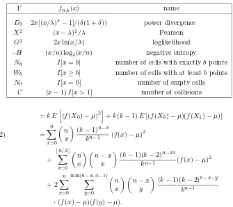
2.1. Choices of fn,k. Some choices offn,k are given in Table 2.1. In each case, Y is a measure of clustering: It tends to increase when the points are less evenly distributed between the cells. The well-known Pearson and loglikelihood statistics, X2 and G2, are both special cases of the power divergence, with δ = 1 and δ→ 0, respectively [39]. H is related toG2via the relationH = log2(k)−G2/(2nln 2). The statisticsNb,Wb, andC count the number of cells that contain exactlyb points (for b≥0), the number of cells that contain at leastbpoints (forb≥1), and the number of collisions (i.e., the number of times a point falls in a cell that already has a point in it), respectively. They are related byN0=k−W1=k−n+C,Wb=Nb+· · ·+Nn, andC=W2+· · ·+Wn.
2.2. Mean and Variance. Before looking at the distribution of Y, we give expressions for computing its exact mean and variance underH0.
If the number of points is fixed at n, (X0, . . . , Xk−1) is multinomial. Denoting
µ=E[fn,k(Xj)], one obtains after some algebraic manipulations:
Table 2.1
Some choices offn,k and the corresponding statistics.
Y fn,k(x) name
Dδ 2x[(x/λ)δ−1]/(δ(1 +δ)) power divergence
X2 (x−λ)2/λ Pearson
G2 2xln(x/λ) loglikelihood
−H (x/n) log2(x/n) negative entropy
Nb I[x=b] number of cells with exactlyb points Wb I[x≥b] number of cells with at leastb points
Although containing a lot of summands, these formulas are practical in the sparse case since for the Y’s defined in Table 2.1, when nand k are large and λ=n/k is small, only the terms for smallxandy in the above sums are non-negligible. These terms converge to 0 exponentially fast as a function ofx+y, whenx+y→ ∞. The first two moments ofY are then easy to compute by truncating the sums after a small number of terms. For example, withn=k= 1000, the relative errors onE[H] and Var[H] are less than 10−10 if the sums are stopped atx, y= 14 instead of 1000, and less than 10−15 if the sums are stopped at x, y= 18. A similar behavior is observed for the other statistics.
The expressions (2.1) and (2.2) are still valid in the dense case, but for largerλ, more terms need to be considered. Approximations for the mean and variance ofDδ whenλ≫1, with error terms ino(1/n), are provided in [39], Chapter 5, page 65.
In the Poisson setup, wherenis the mean of a Poisson random variable, theXj are i.i.d. Poisson(λ) and the expressions become
E[Y] =kµ = k
results are stated in the next proposition. This means that D(δC) and D(δN) in the proposition have exactly the same mean and variance as their asymptotic distribu-tion (e.g., 0 and 1 in the normal case). Read and Cressie [39] recommend this type of standardization, which tends to be closer to the asymptotic distribution than a standardization by the asymptotic mean and variance. The two-moment corrections become increasingly important when δ gets away from around 1. The mean and variance of Dδ can be computed as explained in the previous subsection. Another possibility would be to correct the distribution itself, e.g., using Edgeworth-type ex-pansions [39], page 68. This gives extremely complicated expressions, due in part to the discrete nature of the multinomial distribution, and the gain is small.
Proposition 2.1. Forδ >−1, the following holds underH0. (i) [Dense case] Ifk is fixed andn→ ∞, in the multinomial setup
D(δC)def= Dδ−kµ+ (k−1)σC
σC ⇒
χ2(k−1),
whereσ2
C= Var[Dδ]/(2(k−1)),⇒denotes convergence in distribution, and χ2(k−1) is the chi-square distribution withk−1 degrees of freedom. In the
Poisson setup,D(δC)⇒χ2(k)instead.
(ii) [Sparse case] For both the multinomial and Poisson setups, ifk→ ∞,n→ ∞, andn/k→λ0 where0< λ0<∞, then
D(δN)def= Dδ−kµ σN ⇒
N(0,1),
whereσ2
N = Var[Dδ]andN(0,1)is the standard normal distribution.
Proof. For the multinomial setup, part (i) can be found in [39], page 46, whereas part (ii) follows from Theorem 1 of [11], by noting that all theXj’s here have the same distribution. The proofs simplify for the Poisson setup, due to the independence. The Zj = (Xj−n/k)/
p
n/k are i.i.d. and asymptotically N(0,1) in the dense case, so their sum of squares, which isX2, is asymptoticallyχ2(k).
We now turn to the counting random variables Nb, Wb, and C. These are not approximately chi-square in the dense case. In fact, if n→ ∞for fixed k, it is clear that Nb → 0 with probability 1 for any fixed b. This implies that Wb → k and C→n−k, so these random variables are all degenerate.
For the Poisson setup, eachXi is Poisson(λ), sopb def
= P[Xi =b] =e−λλb/b! for b≥0 andNb is BN(k, pb), a binomial with parametersk andpb. If kis large andpb is small,Nb is thus approximately Poisson with (exact) mean
E[Nb] =kpb= nbe−λ
kb−1b! forb≥0. (2.5)
The next result covers other cases as well.
Proposition 2.2. For the Poisson or the multinomial setup, underH0, suppose
that k→ ∞andn→ ∞, and letλ∞,γ0, andλ0 denote positive constants.
(i) If b≥2 andnb/(kb−1b!)→λ∞, then W
b⇒Nb ⇒Poisson(λ∞). For b= 2, one also has C⇒N2.
(ii) Forb= 0, ifn/k−ln(k)→γ0, thenN0⇒Poisson(e−γ0) .
(iii) If k→ ∞and n/k→λ0>0, then forY =Nb,Wb, orC, Y −E[Y]
Proof. In (i), sinceλ=n/k →0, one has for the Poisson caseE[Nb+1]/E[Nb] = λ/(b+ 1) → 0 and E[Wb+1]/E[Nb] = E[P∞i=1Nb+i]/E[Nb] = P∞i=1λib!/(b+i)! ≤ b!P∞
i=1λi/i! =b!(eλ−1) →0. The relative contribution ofWb+1 to the sumWb = Nb+Wb+1(a sum of correlated Poisson random variables) is then negligible compared with that of Nb, soNb and Wb have the same asymptotic distribution (this follows from Lemma 6.2.2 of [2]). Likewise, under these conditions with b = 2, C has the same asymptotic distribution asN2, becauseC=N2+P∞
i=3(i−1)Ni and therefore eλ−1. For the multinomial setup, it has been shown (see [2], Section 6.2) thatNb andWb, for b≥2, are asymptotically Poisson(kpb) whenλ→0, the same as for the Poisson setup. The same argument as forW2applies forC, using again their Lemma 6.2.2, and this proves (i). Forb = 0, for the Poisson setup, we saw already thatN0 is asymptotically Poisson(λ∞) ifke−n/k→λ∞, i.e., if ln(k)−n/k→ln(λ∞) =−γ0.
For the multinomial case, the same result follows from Theorem 6.D of [2], and this proves (ii). Part (iii) is obtained by applying Theorem 1 of [11].
The exact distributions of C and N0 under H0, for the multinomial setup, are given by
are the Stirling numbers of the second kind (see [13], page 71, where an algorithm is also given to compute all the non-negligible probabilities in timeO(nlogn)).
In our implementation of the test based onC, we used the Poisson approximation for λ ≤1/32, the normal approximation for λ > 1/32 and n >215, and the exact distribution otherwise.
3. Overlapping vectors. For the overlapping case, let Xt,j(o) be the number of overlapping vectorsVi,i= 0, . . . , n−1, that fall into cellj. Now, the formulas (2.1) and (2.2) for the mean and variance, and the limit theorems in Propositions 2.1 and 2.2, no longer stand. The analysis is more difficult than for the disjoint case because in generalP[Xt,i(o)=x] depends oni andP[Xt,i(o)=x, Xt,j(o)=y] depends on the pair (i, j) in a non-trivial way.
Theoretical results have been available in the overlapping multinomial setup, for the Pearson statistic in the dense case. Let
n/k≥5 or so, is called theoverlapping serial test or them-tuple test in the literature and has been used previously to test RNGs (e.g., [1, 29, 30]). The next proposition generalizes the result of Good to the power divergence statistic in the dense case. Further generalization is given by Theorem 4.2 of [43].
Proposition 3.1. Let
the power divergence statistic for the t-dimensional overlapping vectors, and define
˜
Dδ,(t)=Dδ,(t)−Dδ,(t−1). Under H0, in the multinomial setup, ifδ >−1,k is fixed,
andn→ ∞,D˜δ,(t)⇒χ2(dt−dt−1).
Proof. The result is well-known forδ = 1. Moreover, a Taylor series expansion of Dδ,(t) in powers of Xt,j(o)/λ−1 easily shows that Dδ,(t) = D1,(t)+op(1), where op(1) →0 in probability asn→ ∞ (see [39], Theorem A6.1). Therefore, ˜Dδ,(t) has the same asymptotic distribution as ˜D1,(t)and this completes the proof.
For the sparse case, where k, n → ∞ and n/k → λ0 where 0 < λ0 < ∞, our simulation experiments support the conjecture that
˜
The overlapping empty-cells-count test has been discussed in a heuristic way in a few papers. Fort = 2, Marsaglia [30] calls it theoverlapping pairs sparse occupancy
(OPSO) and suggests a few specific parameters, without providing the underlying the-ory. Marsaglia and Zaman [32] speculate thatN0 should be approximately normally distributed with meanke−λand varianceke−λ(1−3e−λ). This make sense only ifλis not too large or not too close to zero. We studied empirically this approximation and found it reasonably accurate only for 2≤λ≤5 (approximately). The approximation could certainly be improved by refining the variance formula.
Proposition 2.2 (i) and (ii) should hold in the overlapping case as well. Our simulation experiments indicate that the Poisson approximation forCis very accurate for (say)λ <1/32, and already quite good forλ≤1, whennis large.
4. Which Test Statistic and What to Expect?. The LFSR, LCG, and MRG generators in our lists are constructed so that their point sets Ψtover the entire period are superuniformly distributed. Thus, we may be afraid, if k is large enough, that very few cells (if any) contain more than 1 point and that Dδ, C, N0, Nb and Wb for b ≥ 2 are smaller than expected. In the extreme case where C = 0, assuming that the distribution of C under H0 is approximately Poisson with mean n2/(2k), the leftp-value of the collision test ispl =P[C ≤0 | H0]≈e−n
2
/(2k). For a fixed number of cells, this p-value approaches 0 exponentially fast in the square of the sample sizen. For example,pl≈3.3·10−4, 1.3·10−14, and 3.4·10−56forn= 4√k, 8√k, and 16√k, respectively. Assuming thatkis near the RNG’s period length, i.e., k≈2e, this means that the test starts to fail abruptly when the sample size exceeds approximately 4 times the square root of the period length. As we shall see, this is precisely what happens for certain popular classes of generators. If we use the statistic Wb instead ofC, in the same situation, we havepl=P[Wb≤0| H0]≈e−n
n=O(k(b−1)/b) forb≥2. In this setup,CandN2are equivalent toW2, and choosing b >2 gives a less efficient test.
Suppose now that we have the opposite: Too many collisions. One simple model of this situation is the alternativeH1: “The points are i.i.d. uniformly distributed over k1boxes, the otherk−k1boxes being always empty.” UnderH1,Wbis approximately Poisson with mean λ1 =nbe−n/k1/(kb−1
1 b!) (if nis large and λ1 is small) instead of λ0 = nbe−n/k/(kb−1b!). Therefore, for a given α0, andx0 such that α0 =P[W
b ≥ x0| H0], the power of the test at levelα0 is
P[Wb≥x0| H1]≈1− x0−1
X
x=0
e−λ1λx
1 x! ,
wherex0depends onb. Whenbincreases, for a fixedα0,x0decreases andλ1decreases as well ifn/k1 ≤b+ 1. So b= 2 maximizes the power unless n/k1 is large. In fact the test can have significant power only if λ1 exceeds a few units (otherwise, with large probability, one has Wb = 0 and H0 is not rejected). This means λ1 =O(1), i.e., n = O(k(1b−1)/b(b!)1/ben/(bk1)), which can be approximated by O(k
(b−1)/b 1 ) if k1 is reasonably large. Then, b = 2 is the best choice. If k1 is small, λ1 is maximized (approximately) by takingb= max(2,⌈n/k1⌉ −1).
The alternativeH1just discussed can be generalized as follows: Suppose that the k1cells have a probability larger than 1/k, while the otherk−k1 cells have a smaller probability. H1is called ahole (resp.,peak,split) alternative ifk1/kis near 1 (resp., near 0, near 1/2). We made extensive numerical experiments regarding the power of the tests under these alternatives and found the following. Hole alternatives can be detected only whenn/k is reasonably large (dense case), because in the sparse case one expects several empty cells anyway. The best test statistics to detect them are those based on the number of empty cellsN0, andDδ withδas small as possible (e.g., −1< δ≤0). For a peak alternative, the power ofDδ increases withδ as a concave function, with a rate of increase that typically becomes very small for δ larger than 3 or 4 (or higher, if the peak is very narrow). The other test statistics in Table 2.1 are usually not competitive withD4(say) under this alternative, except forWb which comes close when b ≈n/k1 (however it is hard to choose the right b because k1 is generally unknown). The split alternative with the probability of the k−k1 low-probability cells equal to 0 is easy to detect and thecollision test (usingC orW2) is our recommendation. The power of Dδ is essentially the same as that ofC and W2, for mostδ, becauseE[W3] has a negligible value, which implies that there is almost a one-to-one correspondence betweenC,W2, andDδ. However, with the smallnthat suffices for detection in this situation, E[W2] is small and the distribution of Dδ is concentrated on a small number of values, so neither the normal nor the chi-square is a good approximation of its distribution. Of course, the power of the test would improve if the high-probability cells were aggregated into a smaller number of cells, and similarly for the low-probability cells. But to do this, one needs to know where these cells area priori.
5. Empirical Evaluation for RNG Families.
5.1. Selected Families of RNGs. We now report systematic experiments to assess the effectiveness of serial tests for detecting the regularities in specific families of small RNGs. The RNG families that we consider are named LFSR3, GoodLCG, BadLCG2, MRG2, CombL2, InvExpl. Within each family, we constructed a list of specific RNG instances, with period lengths near 2e for (integer) values oferanging from 10 to 40. These RNGs are too small to be considered for serious general purpose softwares, but their study gives good indication about the behavior of larger instances from the same families. At stepn, a generator outputs a numberun ∈[0,1).
The LFSR3s are combined linear feedback shift register (LFSR) (or Tausworthe) generators with three components, of the form
xj,n= (arjxj,n−rj +akjxj,n−kj) mod 2, 1≤j ≤3;
uj,n= 32 X
i=1
xj,nsj+i−12
−i, 1
≤j≤3; un=u1,n⊕u2,n⊕u3,n,
where⊕means bitwise exclusive-or, and (kj, rj, sj), 1≤j≤3, are constant parame-ters selected so that thekj are reasonably close to each other, and the sequence{un} has period length (2k1
−1)(2k2
−1)(2k3
−1) and is maximally equidistributed (see [19] for the definition and further details about these generators).
The GoodLCGs are linear congruential generators (LCGs), of the form xn=axn−1 modm; un = xn/m,
(5.1)
where mis a prime near 2eand ais selected so that the period length ism−1 and so that the LCG has an excellent behavior with respect to the spectral test (i.e., an excellent lattice structure) in up to at least 8 dimensions. The BadLCG2s have the same structure, except that their a is chosen so that they have a mediocre lattice structure in 2 dimensions. More details and the values ofa andm can be found in [24, 26]. The MRG2 are multiple recursive generators of order 2, of the form
xn = (a1xn−1+a2xn−2) modm; un = xn/m, (5.2)
period lengthm2−1, and excellent lattice structure as for the GoodLCGs [17, 21]. The CombL2s combine two LCGs as proposed in [15]:
xj,n=ajxj,n−1 modmj, 1≤j≤2; un= ((x1,n+x2,n) mod m1)/m1,
so that the combined generator has period length (m1−1)(m2−1)/2 and an excellent lattice structure (see [28] for details about that lattice structure).
InvExpl denotes a family of explicit inversive nonlinear generators of period length m, defined by
xn = (123n)−1modm; un = xn/m, (5.3)
5.2. The Log-p-values. For a given test statistic Y taking value y, let pl = P[Y ≤y| H0] and pr=P[Y ≥y| H0]. We define thelog-p-value of the test as
ℓ=
k if 10−(k+1)< p
r≤10−k, k >0, −k if 10−(k+1)< p
l≤10−k, k >0, 0 otherwise.
For example,ℓ= 2 means that the rightp-value is between 0.01 and 0.001. For a given class of RNGs, given Y, t, and a way of choosing k, we apply the test for different values ofeand with sample sizen= 2γe+ν, for ν=. . . ,−2,−1,0,1,2, . . ., where the constantγis chosen so that the test starts to fail at approximately the same value of ν for all (or most) e. More specifically, we define ˜ν (resp.ν∗) as the smallest values
ofν for which the absolute log-p-value satisfies|ℓ| ≥2 (resp.|ℓ| ≥14) for a majority of values ofe. These thresholds are arbitrary.
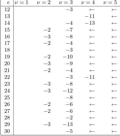
5.3. Test Results: Examples and Summary. Tables 5.1 and 5.2 give the log-p-values for the collision test applied to the GoodLCGs and BadLCG2s, respectively, in t = 2 dimensions, with d = ⌊2e/2⌋ (so k ≈ 2e), and n = 2e/2+ν. Only the log-p-valuesℓ outside of the set{−1,0,1}, which correspond top-values less than 0.01, are displayed. The symbols ←and →mean ℓ≤ −14 andℓ ≥14, respectively. The columns not shown are mostly blank on the left of the table and filled with arrows on the right of the table. The small p-values appear with striking regularity, at about the sameν for alle, in each of these tables. This is also true for other values ofenot shown in the table. One has ˜ν= 2 andν∗= 4 in Table 5.1, while ˜ν=−1 andν∗= 1
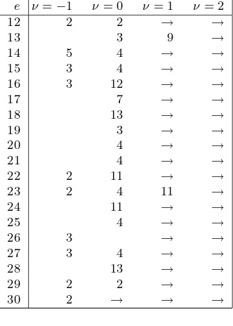
in Table 5.2. The GoodLCGs fail because their structure is too regular (the left p-values are too small because there are too few collisions), whereas the BadLCG2s have the opposite behavior (the right p-values are too small because there are too many collisions; their behavior correspond to thesplit alternative described in Section 4).
Table 5.3 gives the values of ˜ν and ν∗ for the selected RNG families, for the
collision test in 2 and 4 dimensions. All families, except InvExpl, fail at a sample size proportional to the square root of the period lengthρ. At n = 2ν∗
ρ1/2, the left or rightp-value is less than 10−14most of the time. The BadLCG2s in 2 dimensions are the first to fail: They were chosen to be particularly mediocre in 2 dimensions and the test detects it. Apart from the BadLCG2s, the generators always fail the tests due to excessive regularity. For the GoodLCGs and LFSR3s, for example, there was never a cell with more than 2 points in it. For the LFSR3s, we distinguish two cases: One wheredwas chosen always odd and one where it was always the smallest power of 2 such thatk=dt≥2e. In the latter case, the number of collisions is always 0, since no cell contains more than a single point over the entire period of the generator, as a consequence of the “maximal equidistribution” property of these generators [19]. The left p-values then behave as described at the beginning of Section 4. The InvExpl resist the tests until after their period length is exhausted. These generators have their point set Ψt “random-looking” instead of very evenly distributed. However, they are much slower than the linear ones.
Table 5.1
The log-p-valuesℓfor the GoodLCGs with period lengthρ≈2e, for the collision test (based on C), int= 2dimensions, withk≈2e cells, and sample sizen= 2e/2+ν. The table entries give the
values ofℓ. The symbols←and→meanℓ≤ −14andℓ≥14, respectively. Here, we haveν˜= 2
andν∗= 4.
e ν= 1 ν= 2 ν= 3 ν= 4 ν= 5
12 −3 ← ←
13 −11 ←
14 −4 −13 ←
15 −2 −7 ← ←
16 −3 −8 ← ←
17 −2 −4 ← ←
18 −3 ← ←
19 −2 −10 ← ←
20 −3 −9 ← ←
21 −2 −4 ← ←
22 −3 −11 ←
23 −3 −8 ← ←
24 −3 −12 ← ←
25 −8 ← ←
26 −2 −6 ← ←
27 −2 −6 ← ←
28 −2 ← ←
29 −3 −13 ← ←
30 −5 ← ←
overlapping tests are more efficient than the non-overlapping ones, because they call the RNGttimes less.
We applied the same tests with smaller and larger numbers of cells, such as k= 2e/64,k= 2e/8,k= 8·2e, k= 64·2e, and found that ˜ν and ν∗ increase when
k moves away from 2e. A typical example: For the GoodLCGs with t= 2, ν∗ = 7,
6, 5, and 7 for the four choices of k given above, respectively, whereas ν∗ = 4 when
k = 2e. The classical way of applying the serial test for RNG testing uses a large average number of points per cell (dense case). We applied the test based on X2 to the GoodLCGs, with k ≈n/8, and found empirically γ = 2/3, ˜ν = 3, and ν∗ = 4.
This means that the required sample size now increases asO(ρ2/3) instead ofO(ρ1/2) as before; i.e., the dense setup with the chi-square approximation is much less efficient than the sparse setup. We observed the same forDδ with other values ofδand other values oft, and a similar behavior for other RNG families.
For the results just described,twas fixed anddvaried withe. We now fixd= 4 (i.e., we take the first two bits of each number) and vary the dimension ast=⌊e/2⌋. Table 5.4 gives the results of the collision test in this setup. Note the change inγ for the GoodLCGs and BadLCG2s: The tests are less sensitive for these large values of t.
Table 5.2
The log-p-values ℓ for the collision test, with the same setup as in Table 5.1, but for the BadLCG2 generators. Here,˜ν=−1andν∗= 1.
e ν=−1 ν= 0 ν= 1 ν= 2
12 2 2 → →
13 3 9 →
14 5 4 → →
15 3 4 → →
16 3 12 → →
17 7 → →
18 13 → →
19 3 → →
20 4 → →
21 4 → →
22 2 11 → →
23 2 4 11 →
24 11 → →
25 4 → →
26 3 → →
27 3 4 → →
28 13 → →
29 2 2 → →
30 2 → → →
Table 5.3
Collision tests for RNG families, intdimensions, withk≈2e. Recall thatν˜(resp.ν∗) is the smallest integerνfor which|ℓ| ≥2(resp.|ℓ| ≥14) for a majority of values ofe, in tests with sample sizen= 2γe+ν.
RNG family γ t ν˜ ν∗
GoodLCG 1/2 2 2 4
4 3 5
BadLCG2 1/2 2 −1 1
4 3 5
LFSR3,dodd 1/2 2 3 5
4 4 6
LFSR3,dpower of 2 1/2 2 2 4
4 3 4
MRG2 1/2 2 2 4
4 3 5
CombL2 1/2 2 3 5
4 5 7
InvExpl 1 2 1 1
4 1 1
Table 5.4
Collision tests withd= 4divisions in each dimension andt=⌊e/2⌋dimensions.
Generators γ ν˜ ν∗
GoodLCG 2/3 2 3
BadLCG2 2/3 2 4
LFSR3 1/2 2 4
MRG2 1/2 7 8
CombL2 1/2 5 6
InvExpl 1 1 1
technique, for which the required memory is proportional toninstead ofk). Another way of doing a two-level test withDδ is to compute thep-values for theN replicates and compare their distribution with the uniform via (say) a Kolmogorov-Smirnov or Anderson-Darling goodness-of-fit test. We experimented extensively with this as well and found no advantage in terms of efficiency, for all the RNG families that we tried.
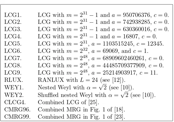
6. What about real-life LCGs?. From the results of the preceding section one can easily predict, conservatively, at which sample size a specific RNG from a given family will start to fail. We verify this with a few commonly used RNGs, listed in Table 6.1. (Of course, this list is far from exhaustive).
Table 6.1
List of selected generators.
LCG1. LCG withm= 231−1 anda= 950706376,c= 0. LCG2. LCG withm= 231−1 anda= 742938285,c= 0. LCG3. LCG withm= 231−1 anda= 630360016,c= 0. LCG4. LCG withm= 231−1 anda= 16807,c= 0. LCG5. LCG withm= 231,a= 1103515245,c= 12345. LCG6. LCG withm= 232,a= 69069, andc= 1. LCG7. LCG withm= 248,a= 68909602460261,c= 0. LCG8. LCG withm= 248,a= 44485709377909,c= 0. LCG9. LCG withm= 248,a= 25214903917,c= 11. RLUX. RANLUX withL= 24 (see [12]).
WEY1. Nested Weyl withα=√2 (see [10]).
WEY2. Shuffled nested Weyl withα=√2 (see [10]). CLCG4. Combined LCG of [25].
CMRG96. Combined MRG in Fig. 1 of [18]. CMRG99. Combined MRG in Fig. 1 of [23].
Table 6.2
The log-p-values for the collision test int= 2dimensions, withk=mcells, and sample size
n= 2ν√m.
Generator ν= 1 ν= 2 ν= 3 ν= 4 ν= 5
LCG1 −2 −11 ← ←
LCG2 −3 −8 ← ←
LCG3 −3 ← ←
LCG4 2 4 → →
LCG5 −3 −13 ← ←
LCG6 −3 −7 ← ←
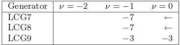
Table 6.3
The log-p-values for the two-level collision test (based onCT) int= 2dimensions, withk= 246
cells, sample sizen= 224+ν for each replication, andN= 32replications.
Generator ν=−2 ν=−1 ν= 0
LCG7 −7 ←
LCG8 −7 ←
LCG9 −3 −3
LCG5), the Numerical Recipes [38], etc., and is suggested in several books and papers (e.g., [3, 36, 40]). LCG6 is used in the VAX/VMS operating system and on Convex computers. LCG5 and LCG9 are the rand and rand48 functions in the standard
libraries of the C programming language [37]. LCG7 is taken from [6] and LCG8 is used in the CRAY system library. LCG1 to LCG4 have period length 231−2, LCG5, LCG6, AND LCG9 have period lengthm, and LCG7 and LCG8 have period length m/4 = 246.
RLUX is the RANLUX generator implemented by James [12], with luxury level L = 24. At this luxury level, RANLUX is equivalent to the subtract-with-borrow generator with modulusb= 232−5 and lagsr= 43 ands= 22 proposed in [31] and used, for example, in MATHEMATICA (according to its documentation). WEY1 is a generator based on the nested Weyl sequence defined by ui = i2αmod 1, where α=√2 (see [10]). WEY2 implements the shuffled nested Weyl sequence proposed in [10], defined byui = ((M i2αmod 1) + 1/2)2αmod 1, with α=
√
2 andM = 12345. CLCG4, CMRG96, and CMRG99 are the combined LCG of [25], the combined MRG given in Figure 1 of [18], and the combined MRG given in Figure 1 of [23].
Table 6.2 gives the log-p-values for the collision test in two dimensions, for LCG1 to LCG6, with k≈m andn= 2ν√m. As expected, suspect values start to appear at sample sizen≈4√m and all these LCGs are definitely rejected withn≈16√m. LCG4 has too many collisions whereas the others have too few. By extrapolation, LCG7 to LCG9 are expected to start failing with n around 226, which is just a bit more than what the memory size of our current computer allowed when we wrote this paper. However, we applied the two-level collision test withN = 32, t= 2,k= 246, andn= 224+ν. Here, the total number of collisionsC
T is approximately Poisson with mean 32n2/(2k)≈64·4ν underH0. The log-p-values are in Table 6.3. With a total sample size of 32·224, LCG7 and LCG8 fail decisively; they have too few collisions. We also tried t = 4, and the collision test with overlapping, and the results were similar.
dimensions. With d = 3, t = 25 (so k = 325), and n = 224, the log-p-value for the collision test is ℓ = 8 (there are 239 collisions, while E[C|H0] ≈ 166). For a two-level test with N = 32, d = 3, t = 25, n = 223, the total number of collisions was CT = 1859, much more than 32E[C|H0] ≈ 1329 (ℓ ≥ 14). This result is not surprising, because for this generator all the pointsVi in 25 dimensions or more lie in a family of equidistant hyperplanes that are 1/√3 apart (see [20, 42]). Note that RANLUX with a larger value of L passes these tests, at least for t ≤ 25. WEY1 passed the tests in 2 dimensions, but failed spectacularly for allt≥3: The points are concentrated in a small number of boxes. For example, with t = 3, k = 1000, and a sample size as small as n = 1024, we observed C = 735 whereasE[C|H0] ≈383 (ℓ≥14). WEY2, CLCG4, CMRG96, and CMRG99 passed all the tests that we tried.
7. Conclusion. We compared several variants of serial tests to detect regulari-ties in RNGs. We found that the sparse tests perform better than the usual (dense) ones in this context. The choice of the functionfn,k does not seem to matter much. In particular, collisions count, Pearson, loglikelihood ratio, and other statistics from the power divergence family perform approximately the same in the sparse case. The overlapping tests require about the same sample size n as the non-overlapping ones to reject a generator. They are more efficient in terms of the quantity of random numbers that need to be generated.
It is not the purpose of this paper to recommend specific RNGs. For that, we refer the reader to [22, 23, 27, 33], for example. However, our test results certainly eliminate many contenders. All LCGs and LFSRs fail these simple serial tests as soon as the sample size exceeds a few times the square root of their period length, regardless of the choice of their parameters. Thus, when their period length is less than 250 or so, which is the case for the LCGs still encountered in many popular software products, they are easy to crack with these tests. These small generators should no longer be used. Among the generators listed in Table 6.1, only the last four pass the tests described in this paper, with the sample sizes that we have tried. All others should certainly be discarded.
REFERENCES
[1] N. S. Altman,Bit-wise behavior of random number generators, SIAM Journal on Scientific and Statistical Computing, 9 (1988), pp. 941–949.
[2] A. D. Barbour, L. Holst, and S. Janson,Poisson Approximation, Oxford Science Publica-tions, Oxford, 1992.
[3] P. Bratley, B. L. Fox, and L. E. Schrage,A Guide to Simulation, Springer-Verlag, New York, second ed., 1987.
[4] I. Csisz´ar,Information type measures of difference of probability distributions and indirect observations, Studia Sci. Math. Hungar., 2 (1967), pp. 299–318.
[5] J. Eichenauer-Herrmann,Inversive congruential pseudorandom numbers: A tutorial, Inter-national Statistical Reviews, 60 (1992), pp. 167–176.
[6] G. S. Fishman, Monte Carlo: Concepts, Algorithms, and Applications, Springer Series in Operations Research, Springer-Verlag, New York, 1996.
[7] G. S. Fishman and L. S. Moore III,An exhaustive analysis of multiplicative congruential random number generators with modulus231
−1, SIAM Journal on Scientific and Statistical Computing, 7 (1986), pp. 24–45.
[8] I. J. Good,The serial test for sampling numbers and other tests for randomness, Proceedings of the Cambridge Philos. Society, 49 (1953), pp. 276–284.
[9] P. E. Greenwood and M. S. Nikulin,A Guide to Chi-Squared Testing, Wiley, New York, 1996.
(1994), pp. 1607–1615.
[11] L. Holst,Asymptotic normality and efficiency for certain goodness-of-fit tests, Biometrika, 59 (1972), pp. 137–145.
[12] F. James, RANLUX: A Fortran implementation of the high-quality pseudorandom number generator of L¨uscher, Computer Physics Communications, 79 (1994), pp. 111–114. [13] D. E. Knuth, The Art of Computer Programming, Volume 2: Seminumerical Algorithms,
Addison-Wesley, Reading, Mass., third ed., 1998.
[14] A. M. Law and W. D. Kelton,Simulation Modeling and Analysis, McGraw-Hill, New York, second ed., 1991.
[15] P. L’Ecuyer, Efficient and portable combined random number generators, Communications of the ACM, 31 (1988), pp. 742–749 and 774. See also the correspondence in the same journal, 32, 8 (1989) 1019–1024.
[16] , Testing random number generators, in Proceedings of the 1992 Winter Simulation Conference, IEEE Press, Dec 1992, pp. 305–313.
[17] ,Uniform random number generation, Annals of Operations Research, 53 (1994), pp. 77– 120.
[18] , Combined multiple recursive random number generators, Operations Research, 44 (1996), pp. 816–822.
[19] ,Maximally equidistributed combined Tausworthe generators, Mathematics of Computa-tion, 65 (1996), pp. 203–213.
[20] , Bad lattice structures for vectors of non-successive values produced by some linear recurrences, INFORMS Journal on Computing, 9 (1997), pp. 57–60.
[21] ,Random number generation, in Handbook of Simulation, J. Banks, ed., Wiley, 1998, pp. 93–137.
[22] , Uniform random number generators, in Proceedings of the 1998 Winter Simulation Conference, IEEE Press, 1998, pp. 97–104.
[23] ,Good parameters and implementations for combined multiple recursive random number generators, Operations Research, 47 (1999), pp. 159–164.
[24] ,Tables of linear congruential generators of different sizes and good lattice structure, Mathematics of Computation, 68 (1999), pp. 249–260.
[25] P. L’Ecuyer and T. H. Andres,A random number generator based on the combination of four LCGs, Mathematics and Computers in Simulation, 44 (1997), pp. 99–107.
[26] P. L’Ecuyer and P. Hellekalek,Random number generators: Selection criteria and testing, in Random and Quasi-Random Point Sets, P. Hellekalek and G. Larcher, eds., vol. 138 of Lecture Notes in Statistics, Springer, New York, 1998, pp. 223–265.
[27] P. L’Ecuyer, R. Simard, E. J. Chen, and W. D. Kelton,An object-oriented random-number package with many long streams and substreams. Submitted, 2001.
[28] P. L’Ecuyer and S. Tezuka,Structural properties for two classes of combined random number generators, Mathematics of Computation, 57 (1991), pp. 735–746.
[29] H. Leeb and S. Wegenkittl,Inversive and linear congruential pseudorandom number gen-erators in empirical tests, ACM Transactions on Modeling and Computer Simulation, 7 (1997), pp. 272–286.
[30] G. Marsaglia,A current view of random number generators, in Computer Science and Statis-tics, Sixteenth Symposium on the Interface, North-Holland, Amsterdam, 1985, Elsevier Science Publishers, pp. 3–10.
[31] G. Marsaglia and A. Zaman, A new class of random number generators, The Annals of Applied Probability, 1 (1991), pp. 462–480.
[32] , Monkey tests for random number generators, Computers Math. Applic., 26 (1993), pp. 1–10.
[33] M. Matsumoto and T. Nishimura,Mersenne twister: A 623-dimensionally equidistributed uniform pseudo-random number generator, ACM Transactions on Modeling and Computer Simulation, 8 (1998), pp. 3–30.
[34] D. Morales, L. Pardo, and I. Vajda,Asymptotic divergence of estimates of discrete distri-butions, Journal of Statistical Planning and Inference, 48 (1995), pp. 347–369.
[35] H. Niederreiter,Random Number Generation and Quasi-Monte Carlo Methods, vol. 63 of SIAM CBMS-NSF Regional Conference Series in Applied Mathematics, SIAM, Philadel-phia, 1992.
[36] S. K. Park and K. W. Miller,Random number generators: Good ones are hard to find, Communications of the ACM, 31 (1988), pp. 1192–1201.
[37] P. J. Plauger,The Standard C Library, Prentice Hall, Englewood Cliffs, New Jersey, 1992. [38] W. H. Press and S. A. Teukolsky, Portable random number generators, Computers in
[39] T. R. C. Read and N. A. C. Cressie,Goodness-of-Fit Statistics for Discrete Multivariate Data, Springer Series in Statistics, Springer-Verlag, New York, 1988.
[40] B. D. Ripley,Thoughts on pseudorandom number generators, Journal of Computational and Applied Mathematics, 31 (1990), pp. 153–163.
[41] M. S. Stephens, Tests for the uniform distribution, in Goodness-of-Fit Techniques, R. B. D’Agostino and M. S. Stephens, eds., Marcel Dekker, New York and Basel, 1986, pp. 331– 366.
[42] S. Tezuka, P. L’Ecuyer, and R. Couture,On the add-with-carry and subtract-with-borrow random number generators, ACM Transactions of Modeling and Computer Simulation, 3 (1994), pp. 315–331.
![05 Planning & Audit Tests[CompatibilityMode]](data:image/gif;base64,R0lGODlhAQABAIAAAP///wAAACH5BAEAAAAALAAAAAABAAEAAAICRAEAOw==)