ADVANCED
Published Titles
APPLIED FUNCTIONAL ANALYSIS
J. Tinsley Oden and Leszek F. Demkowicz
THE FINITE ELEMENT METHOD IN HEAT TRANSFER
AND FLUID DYNAMICS, Second Edition
J.N. Reddy and D.K. Gartling
MECHANICS OF LAMINATED COMPOSITE PLATES:
THEORY AND ANALYSIS
J.N. Reddy
PRACTICAL ANALYSIS OF COMPOSITE LAMINATES
J.N. Reddy and Antonio Miravete
SOLVING ORDINARY and PARTIAL BOUNDARY
VALUE PROBLEMS in SCIENCE and ENGINEERING
Karel Rektorys
CRC Series in
COMPUTATIONAL MECHANICS
and APPLIED ANALYSIS
This book contains information obtained from authentic and highly regarded sources. Reprinted material is quoted with permission, and sources are indicated. A wide variety of references are listed. Reasonable efforts have been made to publish reliable data and information, but the author and the publisher cannot assume responsibility for the validity of all materials or for the consequences of their use.
Neither this book nor any part may be reproduced or transmitted in any form or by any means, electronic or mechanical, including photocopying, microfilming, and recording, or by any information storage or retrieval system, without prior permission in writing from the publisher.
The consent of CRC Press LLC does not extend to copying for general distribution, for promotion, for creating new works, or for resale. Specific permission must be obtained in writing from CRC Press LLC for such copying.
Direct all inquiries to CRC Press LLC, 2000 N.W. Corporate Blvd., Boca Raton, Florida 33431.
Trademark Notice: Product or corporate names may be trademarks or registered trademarks, and are used only for identification and explanation, without intent to infringe.
Visit the CRC Press Web site at www.crcpress.com © 2002 by CRC Press LLC
No claim to original U.S. Government works International Standard Book Number 0-8493-2553-6
Library of Congress Card Number 2001035624 Printed in the United States of America 1 2 3 4 5 6 7 8 9 0
Printed on acid-free paper
Library of Congress Cataloging-in-Publication Data Annamalai, Kalyan.
Advanced thermodynamics engineering / Kalyan Annamalai & Ishwar K. Puri. p. cm. — (CRC series in computational mechanics and applied analysis) Includes bibliographical references and index.
ISBN 0-8493-2553-6 (alk. paper)
1. Thermodynamics. I. Puri, Ishwar Kanwar, 1959- II. Title. III. Series. TJ265 .A55 2001
KA dedicates this text to his mother Kancheepuram Pattammal ram, who could not read or write, and his father, Thakkolam K. Sunda-ram, who was schooled through only a few grades, for educating him in all aspects of his life. He thanks his wife Vasanthal for companionship throughout the cliff–hanging journey to this land of opportunity and his children, Shankar, Sundhar and Jothi for providing a vibrant source of “energy” in his career.
PREFACE
We have written this text for engineers who wish to grasp the engineering physics of thermodynamic concepts and apply the knowledge in their field of interest rather than merely digest the abstract generalized concepts and mathematical relations governing thermodynam-ics. While the fundamental concepts in any discipline are relatively invariant, the problems it faces keep changing. In many instances we have included physical explanations along with the mathematical relations and equations so that the principles can be relatively applied to real world problems.
The instructors have been teaching advanced thermodynamics for more than twelve years using various thermodynamic texts written by others. In writing this text, we acknowl-edge that debt and that to our students who asked questions that clarified each chapter that we wrote. This text uses a “down–to–earth” and, perhaps, unconventional approach in teaching advanced concepts in thermodynamics. It first presents the phenomenological approach to a problem and then delves into the details. Thereby, we have written the text in the form of a self–teaching tool for students and engineers, and with ample example problems. Readers will find the esoteric material to be condensed and, as engineers, we have stressed applications throughout the text. There are more than 110 figures and 150 engineering examples covering thirteen chapters.
Chapter 1 contains an elementary overview of undergraduate thermodynamics, mathematics and a brief look at the corpuscular aspects of thermodynamics. The overview of microscopic thermodynamics illustrates the physical principles governing the macroscopic behavior of substances that are the subject of classical thermodynamics. Fundamental concepts related to matter, phase (solid, liquid, and gas), pressure, saturation pressure, temperature, en-ergy, entropy, component property in a mixture and stability are discussed.
Chapter 2 discusses the first law for closed and open systems and includes problems involving irreversible processes. The second law is illustrated in Chapter 3 rather than pre-senting an axiomatic approach. Entropy is introduced through a Carnot cycle using ideal gas as the medium, and the illustration that follows considers any reversible cycle operating with any medium. Entropy maximization and energy minimization principles are illustrated. Chapter 4 introduces the concept of availability with a simple engineering scheme that is followed by the most general treatment. Availability concepts are illustrated by scaling the performance of various components in a thermodynamic system (such as a power plant or air conditioner) and determining which component degrades faster or outperforms others. Differential forms of energy and mass conservation, and entropy and availability balance equations are presented in Chapters 2 to 4 using the Gauss divergence theorem. The differential formulations allow the reader to determine where the maximum entropy generation or irreversibility occurs within a unit so as to pinpoint the major source of the irreversibility for an entire unit. Entropy genera-tion and availability concepts are becoming more important to energy systems and conserva-tion groups. This is a rapidly expanding field in our energy–conscious society. Therefore, a number of examples are included to illustrate applications to engineering systems. Chapter 5 contains a postulatory approach to thermodynamics. In case the reader is pressed for time, this chapter may be entirely skipped without loss of continuity of the subject.
of stable and metastable states of fluids and where the criteria for stability are violated. Real gas state equations are used to identify the stable and unstable regimes and illustrative exam-ples with physical explanation are given.
Chapter 11 deals with reactive mixtures dealing with complete combustion, flame temperatures and entropy generation in reactive systems. In Chapter 12 criteria for the direc-tion of chemical reacdirec-tions are developed, followed by a discussion of equilibrium calculadirec-tions using the equilibrium constant for single and multi-phase systems, as well as the Gibbs mini-mization method. Chapter 13 presents an availability analysis of chemically reacting systems. Physical explanations for achieving the work equivalent to chemical availability in thermody-namic systems are included. The summary at the end of each chapter provides a brief review of the chapter for engineers in industry.
Exercise problems are placed at the end. This is followed by several tables containing thermodynamic properties and other useful information.
The field of thermodynamics is vast and all subject areas cannot be covered in a sin-gle text. Readers who discover errors, conceptual conflicts, or have any comments, are encour-aged to E–mail these to the authors (respectively, [email protected] and [email protected]). The assistance of Ms. Charlotte Sims and Mr. Chun Choi in preparing portions of the manu-script is gratefully acknowledged. We wish to acknowledge helpful suggestions and critical comments from several students and faculty. We specially thank the following reviewers: Prof. Blasiak (Royal Inst. of Tech., Sweden), Prof. N. Chandra (Florida State), Prof. S. Gollahalli (Oklahoma), Prof. Hernandez (Guanajuato, Mexico), Prof. X. Li. (Waterloo), Prof. McQuay (BYU), Dr. Muyshondt. (Sandia National Laboratories), Prof. Ochterbech (Clemson), Dr. Pe-terson, (RPI), and Prof. Ramaprabhu (Anna University, Chennai, India).
KA gratefully acknowledges many interesting and stimulating discussions with Prof. Colaluca and the financial support extended by the Mechanical Engineering Department at Texas A&M University. IKP thanks several batches of students in his Advanced Thermody-namics class for proofreading the text and for their feedback and acknowledges the University of Illinois at Chicago as an excellent crucible for scientific inquiry and education.
ABOUT THE AUTHORS
Kalyan Annamalai is Professor of Mechanical Engineering at Texas A&M. He received his B.S. from Anna University, Chennai, and Ph.D. from the Georgia Institute of Technology, Atlanta. After his doctoral degree, he worked as a Research Associate in the Division of Engi-neering Brown University, RI, and at AVCO-Everett Research Laboratory, MA. He has taught several courses at Texas A&M including Advanced Thermodynamics, Combustion Science and Engineering, Conduction at the graduate level and Thermodynamics, Heat Transfer, Com-bustion and Fluid mechanics at the undergraduate level. He is the recipient of the Senior TEES Fellow Award from the College of Engineering for excellence in research, a teaching award from the Mechanical Engineering Department, and a service award from ASME. He is a Fel-low of the American Society of Mechanical Engineers, and a member of the Combustion In-stitute and Texas Renewable Industry Association. He has served on several federal panels. His funded research ranges from basic research on coal combustion, group combustion of oil drops and coal, etc., to applied research on the cofiring of coal, waste materials in a boiler burner and gas fired heat pumps. He has published more that 145 journal and conference arti-cles on the results of this research. He is also active in the Student Transatlantic Student Ex-change Program (STEP).
NOMENCLATURE*
Symbol Description SI English Conversion
SI to English
A Helmholtz free energy kJ BTU 0.9478
A area m2 ft2 10.764
a acceleration m s–2 ft s–2 3.281
a specific Helmholtz free energy kJ kg–1 BTU lbm–1 0.4299 a attractive force constant
a specific Helmholtz free energy kJ kmole–1 BTU lbmole–1, 0.4299 b body volume constant m3 kmole–1 ft3 lbmole–1 16.018
c specific heat kJ kg–1 K–1 BTU/lb R 0.2388
COP Coefficient of performance
E energy, (U+KE+PE) kJ BTU 0.9478
ET Total energy (H+KE+PE) kJ BTU 0.9478
e specific energy kJ kg–1 BTU lbm–1 0.4299
eT methalpy = h + ke + pe kJ kg–1 BTU lbm–1 0.4299
F force kN lbf 224.81
f fugacity kPa(or bar) lbf in–2 0.1450
G Gibbs free energy kJ BTU 0.9478
g specific Gibbs free energy kJ kg–1 BTU lbm–1 0.4299 (mass basis)
g gravitational acceleration m s–2 ft s–2 3.281 gc gravitational constant
g Gibbs free energy (mole basis) kJ kmole–1 BTU lbmole–10.4299 ˆg partial molal Gibb's function, kJ kmole–1 BTU lbmole–10.4299
H enthalpy kJ BTU 0.9478
hfg enthalpy of vaporization kJ kg–1 BTU lbm–1 0.4299 h specific enthalpy (mass basis) kJ kg–1 BTU lbm–1 0.4299 ho,h* ideal gas enthalpy kJ kg–1 BTU lbm–1 0.4299
I irreversibility kJ BTU 0.9478
I irreversibility per unit mass kJ kg–1 BTU lbm–1 0.4299
I electrical current amp
ke specific kinetic energy kJ kg–1 BTU lbm–1 0.4299 k ratio of specific heats
L length, height m ft 3.281
l intermolecular spacing m ft 3.281
lm mean free path m ft 3.281
LW lost work kJ BTU 0.9478
LW lost work kJ ft lbf 737.52
M molecular weight, molal mass kg kmole–1 lbm lbmole–1
m 2.2046 Y mass fraction
N number of moles kmole lbmole 2.2046
NAvag Avogadro number molecules molecules 0.4536
kmole–1 lbmole-1 n polytropic exponent in PVn = constant
P pressure kN m–2 kPa lbf in–2 0.1450
PE potential energy kJ BTU 0.9478
pe specific potential energy
Q heat transfer kJ BTU 0.9478
q heat transfer per unit mass kJ kg–1 BTU lb–1 0.4299 qc charge
R gas constant kJ kg–1 K–1 BTU lb–1 R–1 0.2388 R universal gas constant kJ kmole–1 BTU lbmole–10.2388
K–1 R–1
u specific internal energy kJ kg–1 BTU lb–1 0.4299 u internal energy (mole basis) kJ kmole–1 BTU lbmole–10.4299
V volume m3 ft3 35.315
x k mole fraction of species k Y k mass fraction ofspecies k
z elevation m ft 3.281
Z compressibility factor Greek symbols
ˆ
αk activity of component k,
ω specific humidity
ρ density kg m–3 1bm ft–3 0.06243
φ equivalence ratio, fugacity coefficient φ relative humidity,
Φ absolute availability(closed system) kJ BTU 0.9478
Φ' relative availability or exergy kJ kg–1 BTU lb–1 0.4299
φ fugacity coefficient
JT Joule Thomson Coefficient K bar–1 ºR atm–1 1.824 µ chemical potential kJ kmole–1 BTU lbmole–10.4299
ν stoichiometric coefficient
σ entropy generation kJ K–1 BTU R–1 0.2388
Ψ absolute stream availability kJ kg–1 BTU lb–1 0.2388
Ψ' relative stream availability or exergy
Subscripts
max maximum possible work output between two given states (for an expansion process)
m mixture
min minimum possible work input between two given states net net in a cyclic process
p at constant pressure
p,o at constant pressure for ideal gas
v at constant volume
v,o at constant volume for ideal gas
v vapor (Chap. 5)
0 or o ambient, ideal gas state Superscripts
- molal property of k, pure component ^ molal property when k is in a mixure Mathematical Symbols
δ( ) differential of a non-property, e.g., δQ, Wδ , etc. d () differential of property, e.g., du, dh, dU, etc.
RKS Redlich Kwong Soave QS/QE Quasi-equilibrium
ss steady state
sf steady flow
TE, te translational
TER Thermal energy reservoir TM thermo-mechanical equilibrium
TMC Thermo-mechanical-chemical equilibrium
uf uniform flow
us uniform state
VE,ve Vibrational energy
Laws of Thermodynamics in Lay Terminology First Law: It is impossible to obtain something from nothing, but one may break even Second Law: One may break even but only at the lowest possible temperature Third Law: One cannot reach the lowest possible temperature
Implication: It is impossible to obtain something from nothing, so one must optimize resources
The following equations, sometimes called the accounting equations, are useful in the engi-neering analysis of thermal systems.
Accumulation rate of an extensive property B: dB/dt = rate of B entering a volume (˙Bi) – rate of B leaving a volume (˙Be) + rate of B generated in a volume ( ˙Bgen) – rate of B de-stroyed or consumed in a volume (˙Bdes/cons).
Mass conservation: dmcv/dt =m˙i − m˙e.
First law or energy conservation: dEcv/dt =Q˙ −W˙ + m e˙i T i, −m e˙e T e, ,
where eT = h + ke + pe, E = U + KE + PE, δwrev, open = –v dP, δwrev, closed = P dv. Second law or entropy balance equation: dScv/dt =Q T˙ / b + m s˙i i−m s˙e e+ σ˙cv,
where σ˙cv > 0 for an irreversible process and is equal to zero for a reversible process. Availability balance: d E( cv−T So cv/dt =Q(1−T0/TR) + m˙iψi−m˙eψe−W T˙ − oσ˙cv ,
CONTENTS
h. Amount of Matter and Avogadro Number
i. Mixture
1. Explicit and Implicit Functions and Total Differentiation
2. Exact (Perfect) and Inexact (Imperfect) Differentials
a. Mathematical Criteria for an Exact Differential
3. Conversion from Inexact to Exact Form
4. Relevance to Thermodynamics
a. Work and Heat
b. Integral over a Closed Path (Thermodynamic Cycle)
5. Homogeneous Functions
a. Relevance of Homogeneous Functions to Thermodynamics
6. Taylor Series
3. Internal Energy, Temperature, Collision Number and Mean Free Path
a. Internal Energy and Temperature
b. Collision Number and Mean Free Path
4. Pressure
a. Relation between Pressure and Temperature
5. Gas, Liquid, and Solid
7. Heat
11. Properties in Mixtures – Partial Molal Property
E. Summary
2. First Law for a Closed System
a. Mass Conservation
3. First Law for an Open System
a. Conservation of Mass
b. Conservation of Energy
c. Multiple Inlets and Exits
d. Nonreacting Multicomponent System
4. Illustrations
a. Heating of a Residence in Winter
b. Thermodynamics of the Human Body
c. Charging of Gas into a Cylinder
d. Discharging Gas from Cylinders
e. Systems Involving Boundary Work
f. Charging of a Composite System
B. Integral and Differential Forms of Conservation Equations
1. Mass Conservation
3. Second law and Entropy
a. Kelvin (1824-1907) – Planck (1858-1947) Statement
b. Clausius (1822-1888) Statement
C. Consequences of the Second Law
1. Reversible and Irreversible Processes
2. Cyclical Integral for a Reversible Heat Engine
3. Clausius Theorem
7. Relation between ds, δq and T during an Irreversible Process
a. Caratheodary Axiom II
D. Entropy Balance Equation for a Closed System
1. Infinitesimal Form
5. Irreversibility and Entropy of an Isolated System
6. Degradation and Quality of Energy
5. Entropy of a Mixture of Ideal Gases
a. Gibbs–Dalton´s Law
b. Reversible Path Method
F. Local and Global Equilibrium
G. Single–Component Incompressible Fluids
H. Third law
I. Entropy Balance Equation for an Open System
1. General Expression
2. Evaluation of Entropy for a Control Volume
3. Internally Reversible Work for an Open System
4. Irreversible Processes and Efficiencies
5. Entropy Balance in Integral and Differential Form
a. Integral Form
b. Differential Form
a. Steady Flow
b. Solids
J. Maximum Entropy and Minimum Energy
1. Maxima and Minima Principles
a. Entropy Maximum (For Specified U, V, m)
b. Internal Energy Minimum (for specified S, V, m)
c. Enthalpy Minimum (For Specified S, P, m)
d. Helmholtz Free Energy Minimum (For Specified T, V, m)
e. Gibbs Free Energy Minimum (For Specified T, P, m)
2. Generalized Derivation for a Single Phase
a. Special Cases
K. Summary
L. Appendix
1. Proof for Additive Nature of Entropy
2. Relative Pressures and Volumes
B. Optimum Work and Irreversibility in a Closed System
1. Internally Reversible Process
2. Useful or External Work
3. Internally Irreversible Process with no External Irreversibility
a. Irreversibility or Gouy–Stodola Theorem
4. Nonuniform Boundary Temperature in a System
C. Availability Analyses for a Closed System
1. Absolute and Relative Availability under Interactions with Ambient
2. Irreversibility or Lost Work
a. Comments
D. Generalized Availability Analysis
1. Optimum Work
2. Lost Work Rate, Irreversibility Rate, Availability Loss
3. Availability Balance Equation in Terms of Actual Work
a. Irreversibility due to Heat Transfer
4. Applications of the Availability Balance Equation
5. Gibbs Function
b. Availability or Exergetic (Work Potential) Efficiency
2. Heat Pumps and Refrigerators
a. Coefficient of Performance
3. Work Producing and Consumption Devices
a. Open Systems:
4. Graphical Illustration of Lost, Isentropic, and Optimum Work
5. Flow Processes or Heat Exchangers
a. Significance of the Availability or Exergetic Efficiency
b. Relation between ηAvail,f and ηAvail,0 for Work Producing Devices
F. Chemical Availability
1. Closed System
2. Open System
a. Ideal Gas Mixtures
b. Vapor or Wet Mixture as the Medium in a Turbine
c. Vapor–Gas Mixtures
D. Generalized Relation for All Work Modes
1. Electrical Work
6. State Relationships for Real Gases and Liquids
A. Introduction
2. Van der Waals (VW) Equation of State
a. Clausius–I Equation of State
b. VW Equation
4. Other Two–Parameter Equations of State
5. Compressibility Charts (Principle of Corresponding States)
6. Boyle Temperature and Boyle Curves
a. Critical Compressibility Factor (Zc) Based Equations
b. Pitzer Factor
c. Evaluation of Pitzer factor,ω
9. Other Three Parameter Equations of State
a. One Parameter Approximate Virial Equation
b. Beatie – Bridgemann (BB) Equation of State
c. Modified BWR Equation
d. Relation for Densities of Saturated Liquids and Vapors
e. Lyderson Charts (for Liquids)
2. Another Explanation for the Attractive Force
3. Critical Temperature and Attraction Force Constant
2. Internal Energy (du) Relation
6. Gibbs Free Energy or Chemical Potential
7. Fugacity Coefficient
F. Pitzer Effect
1. Generalized Z Relation
G. Kesler Equation of State (KES) and Kesler Tables
H. Fugacity
a. Helmholtz Free Energy A at specified T, V and m
b. G at Specified T, P and m
2. Real Gas Equations
a. Graphical Solution
b. Approximate Solution
3. Heat of Vaporization
4. Vapor Pressure and the Clapeyron Equation
a. Remarks
5. Empirical Relations
a. Saturation Pressures
b. Enthalpy of Vaporization
6. Saturation Relations with Surface Tension Effects
4. Inversion Curves
a. State Equations
b. Enthalpy Charts
c. Empirical Relations
5. Throttling of Saturated or Subcooled Liquids
6. Throttling in Closed Systems
7. Euken Coefficient – Throttling at Constant Volume
a. Physical Interpretation
4. Relationship Between Molal and Pure Properties
a. Binary Mixture
b. Multicomponent Mixture
5. Relations between Partial Molal and Pure Properties
a. Partial Molal Enthalpy and Gibbs function
b. Differentials of Partial Molal Properties
b. Approximate Solutions for ˆgk
c. Standard States
d. Evaluation of the Activity of a Component in a Mixture
e. Activity Coefficient
f. Fugacity Coefficient Relation in Terms of State Equation for P
g. DuhemÐ Margules Relation
h. Ideal Mixture of Real Gases
j. Relation between Gibbs Function and Enthalpy
k. Excess Property
l. Osmotic Pressure
B. Molal Properties Using the Equations of State
1. Mixing Rules for Equations of State
a. General Rule
b. Kay’s Rule
c. Empirical Mixing Rules 25
d. Peng Robinson Equation of State
e. Martin Hou Equation of State
f. Virial Equation of State for Mixtures
2. Dalton’s Law of Additive Pressures (LAP)
3. Law of Additive Volumes (LAV)
4. Pitzer Factor for a Mixture
5. Partial Molal Properties Using Mixture State Equations
a. Kay’s Rule
b. RK Equation of State
C. Summary
9. Phase Equilibrium for a Mixture
A. Introduction
1. Miscible, Immiscible and Partially Miscible Mixture
2. Phase Equilibrium
c. P–T Diagram for a Binary Mixture
d. P–Xk(l)–T diagram
e. Azeotropic Behavior
2. Immiscible Mixture
a. Immiscible Liquids and Miscible Gas Phase
b. Miscible Liquids and Immiscible Solid Phase
a. Single Phase
b. Two Phases
c. Three Phases
d. Theory
2. General Phase Rule for Multicomponent Fluids
3. Raoult’s Law for the Vapor Phase of a Real Gas
10. Stability
e. System with Specified Values of S, V, and m
f. Perturbation in Entropy at Specified Volume
g. Perturbation in Entropy and Volume
h. System with Specified Values of S, P, and m
i. System with Specified Values of T, V, and m
j. System with Specified Values of T, P, and m
k. Multicomponent Systems
C. Application to Boiling and Condensation
1. Physical Processes and Stability
a. Physical Explanation
2. Constant Temperature and Volume
3. Specified Values of S, P, and m
4. Specified Values of S (or U), V, and m
D. Entropy Generation during Irreversible Transformation
E. Spinodal Curves
1. Single Component
2. Multicomponent Mixtures
F. Determination of Vapor Bubble and Drop Sizes
G. Universe and Stability
2. Reaction with Excess Air (Lean Combustion)
3. Reaction with Excess Fuel (Rich Combustion)
1. First Law
2. Adiabatic Flame Temperature
a. Steady State Steady Flow Processes in Open Systems
b. Closed Systems
E. Combustion Analyses In the case of Nonideal Behavior
1. Pure Component
2. Mixture
F. Second Law Analysis of Chemically Reacting Systems
1. Entropy Generated during an Adiabatic Chemical Reaction
2. Entropy Generated during an Isothermal Chemical Reaction
G. Mass Conservation and Mole Balance Equations
1. Steady State System
3. Mathematical Criteria for a Closed System
4. Evaluation of Properties during an Irreversible Chemical Reaction
a. Nonreacting Closed System
b. Reacting Closed System
c. Reacting Open System
5. Criteria in Terms of Chemical Force Potential
6. Generalized Relation for the Chemical Potential
C. Chemical Equilibrium Relations
1. Nonideal Mixtures and Solutions
a. Standard State of an Ideal Gas at 1 Bar
b. Standard State of a Nonideal Gas at 1 Bar
2. Reactions Involving Ideal Mixtures of Liquids and Solids
3. Ideal Mixture of Real Gases
4. Ideal Gases
8. Adiabatic Flame Temperature with Chemical Equilibrium
a. Steady State Steady Flow Process
B. Entropy Generation Through Chemical Reactions
C. Availability
2. Adiabatic Combustion
3. Maximum Work Using Heat Exchanger and Adiabatic Combustor
4. Isothermal Combustion
5. Fuel Cells
a. Oxidation States and electrons
b. H2-O2 Fuel Cell
D. Fuel Availability
E. Summary
14. Problems
A. Chapter 1 Problems
B. Chapter 2 Problems
C. Chapter 3 Problems
D. Chapter 4 Problems
E. Chapter 5 Problems
F. Chapter 6 Problems
G. Chapter 7 Problems
H. Chapter 8 Problems
I. Chapter 9 Problems
J. Chapter 10 Problems
K. Chapter 11 Problems
L. Chapter 12 Problems
M. Chapter 13 Problems
Appendix A. Tables
Appendix B. Charts
Appendix C. Formulae
Chapter 1
1. INTRODUCTION
A. IMPORTANCE, SIGNIFICANCE AND LIMITATIONS
Thermodynamics is an engineering science topic,which deals with the science of “motion” (dynamics) and/or the transformation of “heat” (thermo) and energy into various other energy–containing forms. The flow of energy is of great importance to engineers in-volved in the design of the power generation and process industries. Examples of analyses based on thermodynamics include:
The transfer or motion of energy from hot gases emerging from a burner to cooler water in a hot–water heater.
The transformation of the thermal energy, i.e., heat, contained in the hot gases in an auto-mobile engine into mechanical energy, namely, work, at the wheels of the vehicle.
The conversion of the chemical energy contained in fuel into thermal energy in a com-bustor.
Thermodynamics provides an understanding of the nature and degree of energy trans-formations, so that these can be understood and suitably utilized. For instance, thermodynam-ics can provide an understanding for the following situations:
In the presence of imposed restrictions it is possible to determine how the properties of a system vary, e.g.,
The variation of the temperature T and pressure P inside a closed cooking pot upon heat addition can be determined. The imposed restriction for this process is the fixed volume V of the cooker, and the pertinent system properties are T and P.
It is desirable to characterize the variation of P and T with volume V in an automobile en-gine. During compression of air, if there is no heat loss, it can be shown that PV1.4≈ con-stant (cf. Figure 1).
Inversely, for a specified variation of the system properties, design considerations may re-quire that restrictions be imposed upon a system, e.g.,
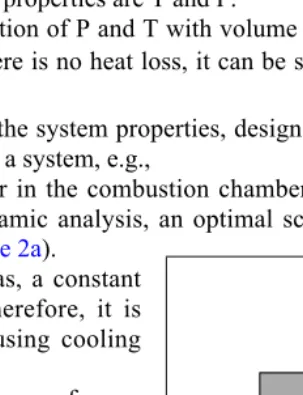
A gas turbine requires compressed air in the combustion chamber in order to ignite and burn the fuel. Based on a thermodynamic analysis, an optimal scenario requires a com-pressor with negligible heat loss (Figure 2a).
During the compression of natural gas, a constant temperature must be maintained. Therefore, it is necessary to transfer heat, e.g., by using cooling assist in making the appropriate decision based on rational scientific bases.
The properties of a substance can be determined using the relevant state equations. Ther-modynamic analysis also provides relations among nonmeasurable properties such as en-ergy, in terms of measurable properties like P and T (Chapter 7). Likewise, the stability of a substance (i.e., the formation of solid, liquid, and vapor phases) can be determined under given conditions (Chapter 10).
Information on the direction of a process can also be obtained. For instance, analysis shows that heat can only flow from higher temperatures to lower temperatures, and chemical reactions under certain conditions can proceed only in a particular direction (e.g., under certain conditions charcoal can burn in air to form CO and CO2, but the reverse process of forming charcoal from CO and CO2 is not possible at those conditions).
B. LIMITATIONS OF THERMODYNAMICS
It is not possible to determine the rates of transport processes using thermodynamic analyses alone. For example, thermodynamics demonstrates that heat flows from higher to lower temperatures, but does not provide a relation for the heat transfer rate. The heat conduc-tion rate per unit area can be deduced from a relaconduc-tion familiarly known as Fourier’s law, i.e.,
˙′′
q = Driving potential ÷ Resistance = ∆T/RH, (1)
where ∆T is the driving potential or temperature difference across a slab of finite thickness, and RH denotes the thermal resistance. The Fourier law cannot be deduced simply with knowl-edge of thermodynamics. Rate processes are discussed in texts pertaining to heat, mass and momentum transport.
1. Review
a. System and Boundary
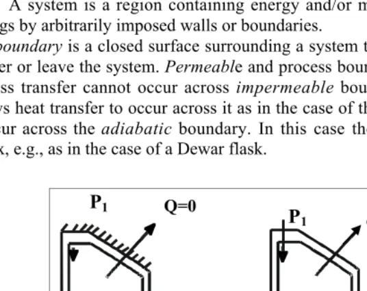
A system is a region containing energy and/or matter that is separated from its sur-roundings by arbitrarily imposed walls or boundaries.
A boundary is a closed surface surrounding a system through which energy and mass may enter or leave the system. Permeable and process boundaries allow mass transfer to occur. Mass transfer cannot occur across impermeable boundaries. A diathermal boundary al-lows heat transfer to occur across it as in the case of thin metal walls. Heat transfer cannot occur across the adiabatic boundary. In this case the boundary is impermeable to heat flux, e.g., as in the case of a Dewar flask.
P
1 QStorage tanks To Combustion
Chamber
P
1 Q=0P 2>P 1 T 2>T 1 P 2>P 1, T 2=T 1
A moveable/deforming boundary is capable of performing “boundary work”.
No boundary work transfer can occur across a rigid boundary. However energy transfer can still occur via shaft work, e.g., through the stirring of fluid in a blender.
A simple system is a homogeneous, isotropic, and chemically inert system with no exter-nal effects, such as electromagnetic forces, gravitatioexter-nal fields, etc.
Surroundings include everything outside the system (e.g. dryer may be a system; but the surroundings are air in the house + lawn + the universe)
An isolated system is one with rigid walls that has no communication (i.e., no heat, mass, or work transfer) with its surroundings.
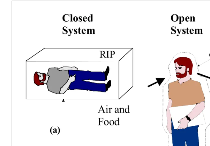
A closed system is one in which the system mass cannot cross the boundary, but energy can, e.g., in the form of heat transfer. Figure 3a contains a schematic diagram of a closed system consisting of a closed–off water tank. Water may not enter or exit the system, but heat can . A philosophical look into closed system is given in Figure 4a.
An open system is one in which mass can cross the system boundary in addition to energy (e.g., as in Figure 3b where upon opening the valves that previously closed off the water tank, a pump now introduces additional water into the tank, and some water may also flow out of it through the outlet).
A composite system consists of several subsystems that have one or more internal con-straints or recon-straints. The schematic diagram contained in Figure 3c illustrates such a sys-tem based on a coffee (or hot water) cup placed in a room. The subsyssys-tems include water (W) and cold air (A)
b. Simple System
A simple system is one which is macroscopically homogeneous and isotropic and involves a single work mode. The term macroscopically homogeneous implies that properties such as the density ρ are uniform over a large dimensional region several times larger than the mean free path (lm) during a relatively large time period, e.g., 10–6 s (which is large compared to the intermolecular collision time that, under standard conditions, is approximately 10–15 s, as we will discuss later in this chapter). Since,
ρ = mass ÷ volume, (2)
where the volume V » lm3, the density is a macroscopic characteristic of any system. System
Boundary
Control Volume
(a) (b) (c)
Hot Water
(W)
Room air
(A)
An isotropic system is one in which the properties do not vary with direction, e.g., a cy-lindrical metal block is homogeneous in terms of density and isotropic, since its thermal conductivity is identical in the radial and axial directions.
A simple compressible system utilizes the work modes of compression and/or expansion, and is devoid of body forces due to gravity, electrical and magnetic fields, inertia, and capillary effects. Therefore, it involves only volumetric changes in the work term.
c. Constraints and Restraints
Constraints and restraints are the barriers within a system that prevent some changes from occurring during a specified time period.
A thermal constraint can be illustrated through a closed and insulated coffee mug. The in-sulation serves as a thermal constraint, since it prevents heat transfer.
An example of a mechanical constraint is a piston–cylinder assembly containing com-pressed gases that is prevented from moving by a fixed pin. Here, the pin serves as a me-chanical constraint, since it prevents work transfer. Another example is water storage be-hind a dam which acts as a mechanical constraint. A composite system can be formulated by considering the water stores behind a dam and the low–lying plain ground adjacent to the dam.
A permeability or mass constraint can be exemplified by volatile naphthalene balls kept in a plastic bag. The bag serves as a non–porous impermeable barrier that restrains the mass transfer of naphthalene vapors from the bag. Similarly, if a hot steaming coffee mug is capped with a rigid non–porous metal lid, heat transfer is possible whereas mass transfer of steaming vapor into the ambient is prevented.
A chemical constraint can be envisioned by considering the reaction of the molecular ni-trogen and oxygen contained in air to form NO. At room temperature N2 and O2 do not re-act at a significant rate and are virtually inert with respect to each other, since a chemical constraint is present which prevents the chemical reaction of the two species from occur-ring. (Non–reacting mixtures are also referred to as inert mixtures.) The chemical
con-RIP
C.V.Open
System
Closed
System
Air and
Food
Exhaust
and
Excretions
(a)
(b)
straint is an activation energy, which is the energy required by a set of reactant species to chemically react and form products. A substance which prevents the chemical reaction from occurring is a chemical restraint, and is referred to as an anti–catalyst, while catalysts (such as platinum in a catalytic converter which converts carbon monoxide to carbon di-oxide at a rapid rate) promote chemical reactions (or overcome the chemical restraint).
d. Composite System
A composite system consists of a combination of two or more subsystems that exist in a state of constrained equilibrium. Using a cup of coffee in a room as an analogy for a com-posite system, the coffee cup is one subsystem and room air another, both of which might exist at different temperatures. The composite system illustrated in Figure 3c consists of two sub-systems hot water (W) and air (A) under constraints, corresponding to different temperatures.
e. Phase
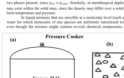
A region within which all properties are uniform consists of a distinct phase. For in-stance, solid ice, liquid water, and gaseous water vapor are separate phases of the same chemi-cal species. A portion of the Arctic Ocean in the vicinity of the North Pole is frozen and con-sists of ice in a top layer and liquid water beneath it. The atmosphere above the ice contains some water vapor. The density of water in each of these three layers is different, since water exists in these layers separately in some combination of three (solid, liquid, and gaseous) phases. Although a vessel containing immiscible oil and water contains only liquid, there are two phases present, since ρoil ≠ρwater. Similarly, in metallurgical applications, various phases may exist within the solid state, since the density may differ over a solid region that is at a uni-form temperature and pressure.
In liquid mixtures that are miscible at a molecular level (such as those of alcohol and water for which molecules of one species are uniformly intermixed with those of the other), even though the mixture might contain several chemical components, a single phase exists,
N2
Pressure Cooker
Vapor, H
2O,ρρρρ
~0.6kg/m
3Liquid , H
2O,ρρρρ
~1000 kg/m
3O2
(a)
(b)
since the system properties are macroscopically uniform throughout a given volume. Air, for example, consists of two major components (molecular oxygen and nitrogen) that are chemi-cally distinct, but constitute a single phase, since they are well–mixed.
f. Homogeneous
A system is homogeneous if its chemical composition and properties are macroscopi-cally uniform. All single–phase substances, such as those existing in the solid, liquid, or vapor phases, qualify as homogeneous substances. Liquid water contained in a cooking pot is a ho-mogeneous system (as shown in Figure 5a), since its composition is the same everywhere, and, consequently, the density within the liquid water is uniform. However, volume contained in the entire pot does not qualify as a homogeneous system even though the chemical composition is uniform, since the density of the water in the vapor and liquid phases differs.
The water contained in the cooker constitutes two phases, liquid and vapor. The molecules are closely packed in the liquid phase resulting in a higher density relative to vapor, and possess lower energy per unit mass compared to that in the vapor phase.
Single–phase systems containing one or more chemical components also qualify as homogeneous systems. For instance, as shown in Figure 5b, air consists of multiple compo-nents but has spatially macroscopic uniform chemical composition and density.
g. Pure Substance
A pure substance is one whose chemical composition is spatially uniform. At any temperature the chemical composition of liquid water uniformly consists of H2O molecules. On the other hand, the ocean with its salt–water mixture does not qualify as a pure substance, since it contains spatially varying chemical composition. Ocean water contains a nonuniform fraction of salt depending on the depth. Multiphase systems containing single chemical com-ponents consist of pure substances, e.g., a mixture of ice, liquid water, and its vapor, or the
Water & alcohol
(vap) 20:80
Water and alcohol
(liq) 40:60
Alcohol
( )
Alcohol (liq)
Water(liq)
Water(g)
liquid water and vapor mixture in the cooking pot example (cf. Figure 5a). Multicomponent single–phase systems also consist of pure substances, e.g., air (cf. Figure 5b).
Heterogeneous systems may hold multiple phases (e.g., as in Figure 5a with one com-ponent) and multicomponents in equilibrium (e.g., Figure 6 with two components). Well–mixed single–phase systems are simple systems although they may be multicomponent, since they are macroscopically homogeneous and isotropic, e.g., air. The vapor–liquid system illustrated in Figure 6 does not qualify as a pure substance, since the chemical composition of the vapor differs from that of the liquid phase.
h. Amount of Matter and Avogadro Number
Having defined systems and the types of matter contained within them (such as a pure, single phase or multiphase, homogeneous or heterogeneous substance), we will now de-fine the units employed to measure the amount of matter contained within systems.
The amount of matter contained within a system is specified either by a molecular number count or by the total mass. An alternative to using the number count is a mole unit. Matter consisting of 6.023×1026 molecules (or Avogadro number of molecules) of a species is called one kmole of that substance. The total mass of those molecules (i.e., the mass of 1 kmole of the matter) equals the molecular mass of the species in kg. Likewise, 1 lb mole of a species contains its molecular mass in lb. For instance, 18.02 kg of water corresponds to 1 kmole, 18.02 g of water contains 1 gmole, while 18.02 lb mass of water has 1 lb mole of the substance. Unless otherwise stated, throughout the text the term mole refers to the unit kmole.
i. Mixture
A system that consists of more than a single component (or species) is called a mix-ture. Air is an example of a mixture containing molecular nitrogen and oxygen, and argon. If Nk denotes the number of moles of the k–th species in a mixture, the mole fraction of that spe-cies Xk is given by the relation
Xk = Nk/N, (3)
where N = ΣNk is the total number of moles contained in the mixture. A mixture can also be described in terms of the species mass fractions mfk as
Yk = mk/m, (4)
where mk denotes the mass of species k and m the total mass. Note that mk = NkMk, with the symbol Mk representing the molecular weight of any species k. Therefore, the mass of a mix-ture
m = ΣNkMk.
The molecular weight of a mixture M is defined as the average mass contained in a kmole of the mixture, i.e.,
M = m/N = ΣNkMk/N = ΣXkMk (5)
a. Example 1
Assume that a vessel contains 3.12 kmoles of N2, 0.84 kmoles of O2, and 0.04 kmoles of Ar. Determine the constituent mole fractions, the mixture molecular weight, and the spe-cies mass fractions.
Solution
Total number of moles N = 3.12 + 0.84 + 0.04 = 4.0 kmoles
The total mass m = 3.12×28.02 + 0.84×32 + 0.04×39.95 = 115.9 kg, and mass fractions are:
YN2 = mN2/m = 3.12×28.02/115.9 = 0.754. Similarly YO2 = 0.232, and YAr = 0.0138.
Remark
The mixture of N2, O2, and Ar in the molal proportion of 78:1:21 is representative of the composition of air (see the Appendix to this chapter).
When dealing specifically with the two phases of a multicomponent mixture, e.g., the alcohol–water mixture illustrated in Figure 6, we will denote the mole fraction in the gaseous phase by Xk,g (often simply as Xk) and use Xk,l Xk,s to represent the liquid and solid phase mole fraction, respectively.
At room temperature (of 20ºC) it is possible to dissolve only up to 36 g of salt in 100 g of water, beyond which the excess salt settles. Therefore, the mass fraction of salt in water at its solubility limit is 27%. At this limit a one–phase saline solution exists with a uniform den-sity of 1172 kg m–3. As excess salt is added, it settles, and there are now two phases, one con-taining solid salt (ρ = 2163 kg m–3) and the other a liquid saline solution (ρ = 1172 kg m–3). (Recall that a phase is a region within which the properties are uniform.)
Two liquids can be likewise mixed at a molecular level only within a certain range of concentrations. If two miscible liquids, 1 and 2, are mixed, up to three phases may be formed in the liquid state: (1) a miscible phase containing liquids 1 and 2 with ρ = ρmixture, (2) that containing pure liquid 1 (ρ = ρ1), and (3) pure liquid 2 (ρ = ρ2). A more detailed discussion is presented in Chapter 8.
j. Property
Thus far we have defined systems, and the type and amount of matter contained within them. We will now define the properties and state of matter contained within these sys-tems.
A property is a characteristic of a system, which resides in or belongs to it, and it can be assigned only to systems in equilibrium. Consider an illustration of a property the tem-perature of water in a container. It is immaterial how this temtem-perature is reached, e.g., either through solar radiation, or electrical or gas heating. If the temperature of the water varies from, say, 40ºC near the boundary to 37ºC in the center, it is not single–valued since the system is not in equilibrium, it is, therefore, not a system property. Properties can be classified as fol-lows:
Primitive properties are those which appeal to human senses, e.g., T, P, V, and m.
Derived properties are obtained from primitive properties. For instance, the units for force (a derived property) can be obtained using Newton’s second law of motion in terms of the fundamental units of mass, length and time. Similarly, properties such as enthalpy H, en-tropy S, and internal energy U, which do not directly appeal to human senses, can be de-rived in terms of primitive properties like T, P and V using thermodynamic relations (Chapter VII). (Even primitive properties, such as volume V, can be derived using state relations such as the ideal gas law V = mRT/P.)
Intensive properties are independent of the extent or size of a system, e.g., P (kN m–2), v (m3 kg–1), specific enthalpy h (kJ kg–1), and T (K).
Extensive properties depend upon system extent or size, e.g., m (kg), V (m3), total en-thalpy H (kJ), and total internal energy U (kJ).
An extrinsic quantity is independent of the nature of a substance contained in a system (such as kinetic energy, potential energy, and the strength of magnetic and electrical fields).
Intensive and extensive properties require further discussion. For example, consider a vessel of volume 10 m3 consisting of a mixture of 0.32 kmoles of N2, and 0.08 kmoles of O2 at 25ºC (system A), and another 15 m3 vessel consisting of 0.48 kmoles of N2 and 0.12 kmoles of O2 at the same temperature (system B). If the boundary separating the two systems is removed, the total volume becomes 25 m3 containing 0.8 total moles of N2, and 0.2 of O2. Properties which are additive upon combining the two systems are extensive, e.g., V, N, but intensive properties such as T and P do not change. Likewise the mass per unit volume (density) does not change upon combining the two systems, even though m and V increase. The kinetic en-ergy of two moving cars is additive m1V12/2 + m2V22/2 as is the potential energy of two masses at different heights (such as two ceiling fans of mass m1 and m2 at respective heights Z1 and Z2 with a combined potential energy m1gZ1 + m2gZ2). Similarly, other forms of energy are addi-tive.
An extensive property can be converted into an intensive property provided it is dis-tributed uniformly throughout the system by determining its value per unit mass, unit mole, or unit volume. For example, the specific volume v = V/m (in units of m3 kg–1) or V/N (in terms of m3 kmole–1). The density ρ = m/V is the inverse of the mass–based specific volume. We will use lower case symbols to denote specific properties (e.g.: v, v, u, and u, etc.). The over-bars denote mole–based specific properties. The exceptions to the lower case rule are tem-perature T and pressure P. Furthermore we will represent the differential of a property as d(property), e.g., dT, dP, dV, dv, dH, dh, dU, and du. (A mathematical analogy to an exact differential will be discussed later.)
k. State
The condition of a system is its state, which is normally identified and described by the observable primitive properties of the system. The system state is specified in terms of its properties so that it is possible to determine changes in that state during a process by monitor-ing these properties and, if desired, to reproduce the system. For example, the normal state of an average person is usually described by a body temperature of 37ºC. If that temperature rises to 40ºC, medication might become necessary in order to return the “system” to its normal state. Similarly, during a hot summer day a room might require air conditioning. If the room tem-perature does not subsequently change, then it is possible to say that the desired process, i.e., air conditioning, did not occur. In both of the these examples, temperature was used to de-scribed an aspect of the system state, and temperature change employed to observe a process. Generally, a set of properties, such as T, V, P,
N1, N2, etc., representing system characteris-tics define the state of a given system.
Figure 7 illustrates the mechanical analogy to various thermodynamic states in a gravitational field. Equilibrium states can be characterized as being stable, metastable, and unstable, depending on their response to a perturbation. Positions A, B and C are at an equilibrium state, while D represents a non-equilibrium position. Equilibrium states can be classified as follows:
A stable equilibrium state (SES), is asso-ciated with the lowest energy, and which, following perturbation, returns to its original state (denoted by A in Figure 7). A closed system is said to achieve a state of stable equilibrium when changes oc-cur in its properties regardless of time, and which returns to its original state
ter being subjected to a small perturbation. The partition of a system into smaller sub–systems has a negligible effect on the SES.
If the system at state B in Figure 7 is perturbed either to the left or right, it reverts back to its original position. However, it appears that a large perturbation to the right is capable of lowering the system to state A. This is an example of a metaequilibrium state (MES). It is known that water can be superheated to 105ºC at 100 KPa without producing vapor bub-bles which is an example of a metastable state, since any impurities or disturbances intro-duced into the water can cause its sudden vaporization (as discussed in Chapter 10). A slight disturbance to either side of an unstable equilibrium state (UES) (e.g., state C of
Figure 7) will cause a system to move to a new equilibrium state. (Chapter 10 discusses the thermodynamic analog of stability behavior.)
The system state cannot be described for a nonequilibrium (NE) position, since it is tran-sient. If a large weight is suddenly placed upon an insulated piston–cylinder system that contains an ideal compressible fluid, the piston will move down rapidly and the system temperature and pressure will continually change during the motion of the piston. Under these transient circumstances, the state of the fluid cannot be described.
Furthermore, various equilibrium conditions can occur in various forms:
Mechanical equilibrium prevails if there are no changes in pressure. For example, helium constrained by a balloon is in mechanical equilibrium. If the balloon leaks or bursts open, the helium pressure will change.
Thermal equilibrium exists if the system temperature is unchanged.
Phase equilibrium occurs if, at a given temperature and pressure, there is no change in the mass distribution of the phases of a substance, i.e., if the physical composition of the sys-tem is unaltered. For instance, if a mug containing liquid water is placed in a room with both the liquid water and room air being at the same temperature and the liquid water level in the mug is unchanged, then the water vapor in the room and liquid water in the mug are in phase equilibrium. A more rigorous definition will be presented later in Chapters 3, 7, and 9.
Chemical equilibrium exists if the chemical composition of a system does not change. For example, if a mixture of H2, O2, and H2O of arbitrary composition is enclosed in a vessel at a prescribed temperature and pressure, and there is no subsequent change in chemical composition, the system is in chemical equilibrium. Note that the three species are allowed to react chemically, the restriction being that the number of moles of a species that are consumed must equal that which are produced, i.e., there is no net change in the concentration of any species (this is discussed in Chapter 12).
The term thermodynamic state refers only to equilibrium states. Consider a given room as a system in which the region near the ceiling consists of hot air at a temperature TB due to relatively hot electrical lights placed there, and otherwise cooler air at a temperature of TA elsewhere. Therefore, a single temperature value cannot be assigned for the entire system, since it is not in a state of thermal equilibrium. However, a temperature value can be specified separately for the two subsystems, since each is in a state of internal equilibrium.
l. Equation of State
Having described systems, and type and state of matter contained within them in terms of properties, we now explore whether all of the properties describing a state are inde-pendent or if they are related.
A thermodynamic state is characterized by macroscopic properties called state vari-ables denoted by x1, x2, … ,xn and F. Examples of state variables include T, P, V, U, H, etc. It has been experimentally determined that, in general, at least one state variable, say F, is not independent of x1, x2, … ,xn, so that
Equation (6) is referred to as a state postulate or state equation. The number of independent variables x1, x2, … ,xn (in this case there are n variables) is governed by the laws of thermody-namics. Later, in Chapter 3, we will prove this generalized state equation. For example, if x1 = T, x2 = V, x3 = N, and F = P, then
P = P (T, V, N).
For an ideal gas, the functional form of this relationship is given by the ideal gas law, i.e.,
P = NRT/V, (7)
whereRis known as the universal gas constant, the value of which is 8.314 kJ kmole–1 K–1. The universal gas constant can also be deduced from the Boltzmann’s constant, which is the universal constant for one molecule of matter (defined as kB =R/NAvog = 1.38×10⁻²⁸ kJ mole-cule–1 K–1). Defining the molar specific volume = V/N, we can rewrite Eq. (7) as
P =RT/v. (8)
Equation (8) (stated by J. Charles and J. Gay Lussac in 1802) is also called an intensive equa-tion of state, since the variables contained in it are intensive. The ideal gas equation of state may be also expressed in terms of mass units after rewriting Eq. (7) in the form
P = (m/M)RT/V = mRT/V (9)
where R =R/M. Similarly,
P = RT/v (10)
Equation (10) demonstrates that P = P (T,v) for an ideal gas and is known once T and v are prescribed. We will show later that this is true for all single–component single–phase fluids.
Consider the composite system containing separate volumes of hot and cold air (as-sumed as ideal gas) at temperatures TA and TB, respectively. We cannot calculate the specific volume for the entire system using Eq. (10), since the temperature is not single valued over the entire system. For a nonequilibrium system, state equations for the entire system are meaning-less. However, the system can be divided into smaller subsystems A and B, with each assumed to be in a state of internal equilibrium. State equations are applicable to subsystems that are in local equilibrium.
m. Standard Temperature and Pressure
Using Eq. (8), it can be shown that the volume of 1 kmole of an ideal gas at standard temperature andpressure (STP), given by the conditions T = 25ºC (77ºF) and P = 1 bar (≈ 1 atm) is 24.78 m3 kmole–1 (392 ft3 lb mole–1,) This volume is known as a standard cubic meter (SCM) or a standard cubic foot (SCF). See the attached tables for the values of volume at various STP conditions.
n. Partial Pressure
The equation of state for a mixture of ideal gases can be generalized if the number of moles in Eq. (7) is replaced by
N = N1 + N2 + N3 + ... = ΣNk, (11)
so that Eq. (7) transforms into
P = N1RT/V + N2RT/V+... (12)
p1 = N1RT/P = X1NRT/V = X1P. (13)
Assuming air at a standard pressure of 101 kPa to consist of 21 mole percent of mo-lecular oxygen, the pressure exerted by O2 molecules alone pO2 is 0.21×101 = 21.21 kPa. Further details of mixtures and their properties will be discussed in Chapters 8 and 9.
o. Process
A process occurs when a system undergoes a change of state (i.e., its properties change) with or without interaction with its surroundings. A spontaneous processchanges the state of a system without interacting with its environment. For instance, if a coffee cup is placed in an insulated rigid room, the properties of the composite system (e.g., Tair, Tcoffee) change with time even though there is no interaction of the room with the outside environment through work or non–work (e.g., heat.) energy transfer.
During an isothermal process there are no temperature changes, i.e., dT = 0. Likewise, for an isobaric process the pressure is constant (dP = 0), and volume remains unchanged during an isometric process (dV = 0). Note that if the temperature difference during a process ∆T = Tf – Tin = 0, this does not necessarily describe an isothermal process, since it is possible that the system was heated from an initial temperature Tin to an intermediate temperature Tint (> Tin) and cooled so that the final temperature Tf = Tin. An adiabatic
process is one during which there is no heat transfer, i.e., when the system is perfectly in-sulated.
If the final state is identical to the initial system state, then the process is cyclical. Other-wise, it is noncyclical.
p. Vapor–Liquid Phase Equilibrium
Having defined systems, matter, and some relations among system properties (in-cluding those for ideal gases), we now discuss various other aspects of pure substances. Con-sider a small quantity of liquid water contained in a piston–cylinder assembly as illustrated in
Figure 8a.
Assume the system temperature and pressure (T,P) to be initially at standard condi-tions. State A shown in Figure 8a is the compressed liquid state (illustrated on the pres-sure–volume diagram of Figure 8b) corresponding to sub–cooled liquid. If the water is heated, a bubble begins to form once the temperature reaches 100ºC (at the bubble point or the satu-rated liquid state, illustsatu-rated by point F in Figure 8b). This temperature is called the saturation temperature or boiling point temperature at the prescribed pressure. The specific volume of the liquid at this saturated state is denoted by vf. As more heat is added, the two liquid and vapor phases coexist at state W (in the two–phase or wet region, v > vf). The ratio of vapor (subscript g) to total mass m is termed quality (x = mg/m). As more heat is added, the liquid completely converts to vapor at state G which is called the saturated vapor state or the dew point. Upon further heat addition at the specified pressure, the system temperature becomes larger than the saturation temperature, and enters state S which is known as the superheated vapor state.
In the context of Figure 8a and b, the symbol A denotes the subcooled liquid or com-pressed liquid state; F the saturated liquid state (it is usual to use the subscript f to represent the system properties of the fluid at that state) for which the quality x = 0. W is the wet state con-sisting of a mixture of liquid and vapor, G a saturated vapor state (denoted with the subscript g, x = 1), and S represents the superheated vapor
The curve AFWGS in Figure 8b describes an isobaric process. If the system pressure for the water system discussed in the context of Figure 8a is changed to, say, 10, 100, 200, and 30,000 kPa, these pressures correspond to different saturation temperatures, liquid and vapor volumes, and isobaric process curves. Joining all possible curves for saturated liquid and vapor states it is possible to obtain the saturated liquid and vapor curves shown in Figure 8b which intersect at the critical point C that corresponds to a distinct critical temperature and pressure Tc and Pc.
The Table A-1 contains critical data for many substances while Tables A-4 contain in-formation regarding the properties of water along the saturated vapor and liquid curves, and in the superheated vapor regions and Table A-5 contains same information for R-134a. A representa-tive P–v diagram and various liquid–vapor regime terminology are illustrated in Figure 8c as follows:
If the vapor temperature T > Tc, and its pressure P < Pc the vapor is called a gas. A gas is a fluid that, upon isothermal compression, does not change phase (i.e., from gas to liquid as in Curve LM, T > Tc). Otherwise, the fluid is called a vapor (a fluid in a vapor state may be compressed to liquid through a process such as along the curve SGWFK).
Substances at P>Pc and T>Tc are generally referred to as fluid (e.g., point U of Figure 8c). If a supercritical fluid is isobarically heated there is no change of phase (e.g., line RU of
Figure 8c).
Above the critical point, i.e., when P>Pc, and T>Tc the vapor is called a fluid which exists in a supercritical state. If P > Pc, and T < Tc it is referred to as a supercritical fluid (region (1), Figure 8c).
A subcritical fluid is one for which P < Pc, T < Tc, and v < vf.
Both liquid and vapor are contained in the two–phase dome where P < Pc, T < Tc, and vf < v < vg.
The saturated liquid line of Figure 8c joins those states that have been denoted by the subscript F in the context of Figure 8a, e.g., points D, F, etc. Likewise, the saturated vapor line joins the states represented by the subscript g, i.e., the points G, E, etc. of Figure 8c. At the critical point C the saturated liquid and vapor states are identical. Upon plotting the pressure with respect to the saturation temperatures Tsat along the saturated curve, the phase diagram of
Figure 8d is obtained. In that figure the vaporization curve is represented by JC, JQ is the melting curve for most solids (JQ´ is the analogous melting curve for ice), and JR represents the sublimation curve. The intersection J of the curves JC and JQ´ is called the triple point at which all three phases co–exist. For water, this point is characterized by P = 0.0061 bar (0.006 atm) and T = 273.16 K (491.7 R), whereas for carbon the analogous conditions are T ≈ 3800 K, P ≈ 1 bar. For triple points of other substances see Table A-2.
C. MATHEMATICAL BACKGROUND
Thus far, we have discussed the basic terminology employed in thermodynamics. We now briefly review the mathematical background required for expressing the conservation equations in differential form (that will be discussed in Chapters. 2, 3 and 4), equilibrium crite-ria (Chapter 3), conversion of the state equations from one form to another (Chapter 5), Max-well’s relations (Chapter 7), the Euler equation (Chapters 3 and 8) stability behavior of fluids (Chapter 10 and entropy maximization and Gibb’s function minimization (Chapters 3 and 12).
1. Explicit and Implicit Functions and Total Differentiation
If P is a known function of T and v, the explicit function for P is
P = P(v,T), (14)
and its total differential may be written in the form
dP P
where a and b are constants. Equation (16) is explicit with respect to P, since it is an explicit function of T and v. On the other hand, v cannot be explicitly solved in terms of P and T, and, hence, it is an implicit function of those variables. The total differential is useful in situations that require the differential of an implicit function, as illustrated below.
b. Example 2
If state equation is expressed in the form
P = RT/(v–b) – a/v2, (A)
find an expression for (∂v/∂T)P, and for the isobaric thermal expansion coefficient βP = (1/v) (∂v/∂T)P.
Solution
For given values of T and v, and the known parameters a and b, values of P are unique (P is also referred to as a point function of T and v). Using total differentiation
dP = (∂P/∂v)T dv + (∂P/∂T)v dT. (B)
From Eq. (A)
(∂P/∂T)v = R/(v – b) (D)
Substituting Eqs.(C) and (D) in Eq. (B) we obtain
dP = (–RT/(v – b)2 + 2a/v3)
T dv + (R/(v – b))v dT. (E) We may use Eq. (E) to determine (∂v/∂T)P or (∂v /∂P)T. At constant pressure, Eq. (E) yields
0 = (–RT/(v – b)2 + 2a/v3)T dv + (R/(v – b))v dT, (F)
so that
(∂vP /∂TP) = (∂v/∂T)P = –(R/(v – b))/(–RT/(v – b)2 + 2a/v3), (G)
and the isobaric compressibility
βP = 1/v (∂v/∂T)P = –R/(v(–RT/(v–b) + 2a(v–b)/v3)). (H)
Remarks
It is simple to obtain (∂P/∂T)v or (∂P/∂v)T from Eq. (A). It is difficult, however, to obtain values of (∂v/∂T)P or (∂v/∂P)T from that relation. Therefore, the total differentiation is em-ployed.
Note that Eqs. (C) and (D) imply that for a given state equation:
(∂P/∂T)v = M(T,v), and (I)
(∂P/∂v)T = N(T,v), and (J)
Since,
dP = M(T,v) dv + N(T,v) dT, (K)
Differentiating Eq. (C) with respect to T,
∂/∂T (∂P/∂v) = (∂M/∂T)v = –R/(v – b)2. (L)
Likewise, differentiating Eq. (D) with respect to v,
∂/∂v (∂P/∂T) = (∂N/∂v)T = –R/(v – b)2. (M)
From Eqs. (L) and (M) we observe that
∂M/∂T = ∂N/∂v or ∂2P/∂T∂v = ∂2P/∂v∂T. (N)
Eq. (N) illustrates that the order of differentiation does not alter the result. The equation applies to all state equations or, more generally, to all point functions (see next section for more details).
From Eq. (B), at a specified pressure
(∂P/∂v)Tdv + (∂P/∂T)vdT = M(T,v) dv + N(T,v) dT = 0.
Therefore,
(∂v/∂T)P = –M(T,v)/N(T,v) = –(∂P/∂T)v/(∂P/∂v)T. (O)
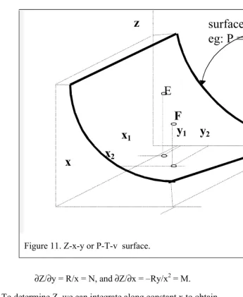
Eq. (O) can be rewritten in the form