Applications of boundary integral equation methods in 3D
electromagnetic scattering
1Department of Mathematical Sciences, University of Delaware, Newark, DE 19716, USA
G.C. Hsiao∗, R.E. Kleinman, D.-Q. Wang
Received 17 June 1998
Abstract
This paper is concerned with the application of boundary integral equation method to the electromagnetic scattering of a perfect conductor in the three dimensional space. A collocation method is employed for the magnetic eld integral equation and error estimates are derived. Far-eld patterns and radar cross sections are computed for various wave numbers in the case of sphere. Numerical experiments are compared to those ontained from the Mie series method in order to verify the predicted theoretical results. c1999 Published by Elsevier Science B.V. All rights reserved.
Keywords:Maxwell’s equations; Scattering; Boundary integral equation; Far-eld pattern
1. Introduction
Boundary integral equation methods have played a major role in the numerical solution of Maxwell’s equations for over three decades. The exact formulation of the boundary integral equations for the physical problems in exterior domains is especially suitable for electromagnetic scattering. Compared to the classical Mie series method, it allows more exible geometry of the obstacles and a variety of incident waves.
While tremendous strides have been taken over the years, many problems remain intractable due to the large size of the scattering objects and the oscillation of the kernels in the integral equations. One of these problems concerns the accuracy of approximate solutions. In a recent series of papers [4–7, 9, 18], an attempt has been made in the context of integral equations for scalar two dimensional problems.
∗Corresponding author. Fax: +1-302-831-4511; e-mail: [email protected] (G.C. Hsiao)
1This work was supported by the Air Force Oce of Scientic Research, Air Force Material Command, USAF, under Grant F9620-96-1-10039. The views and conclusions contained herein are those of authors and should not be intepreted as necessarily representing the ocial policies or endorsements, either expressed or implied, of the Air Force Oce of Scientic Research or the US government.
Very little rigorous analysis for electromagnetic scattering in three dimensions is available. We only know of the method of residual analysis in Sobolev spaces [8] and covolume schemes for time dependent Maxwell’s equations [12, 13]. Our goal in this paper is to provide a rigorous proof of convergence in terms of mesh sizes for the magnetic eld integral equations (MFIE) applied to the electromagnetic scattering of a perfect conductor in the three-dimensional space. The corresponding analysis for the transmission problems will be given in a subsequent report.
The contents of this paper are as follows: we begin Section 2 with an integral formulation for electromagnetic scattering of a perfect conductor object. Following that is a section on numerical discretizations of the MFIE. The numerical scheme used is the collocation method. Section 4 contains the main result, an error estimate for the numerical approximation. In the last section, Section 5, numerical experiments are performed and compared to those obtained from the Mie series method. These numerical results verify the error estimate in the previous sections.
2. Integral representations
Let − be a convex bounded domain in R3 with twice continuously dierentiable boundary and unit normal n pointing to the exterior domain. Let + denote the exterior of −. Then if (E+(x);H+(x)) and (E−(x);H−(x)) denote, respectively, electromagnetic eld in + and −, the source free Maxwell’s equations [3] are
curl E+= ikZH+; curl H+=−ikYE+ in +; (2.1)
uniformly for all directions x=|x|. In (2.1) and (2.2), k denotes the wave number and
Z= 1=Y=p
1
The classical jump conditions [3] state that if n·E± are Holder continuous on
lim
− denotes Cauchy principal value integral. A similar result holds for n·H±. Moreover, if
n×E± are Holder continuous on , then
y are continuous as x → ± with no jumps and the resulting boundary integrals have weakly singular kernels. These jump conditions remain valid in dierent senses with weaker conditions on densities, see [8] for details.
Combining these limiting values with the representations (2.4) and (2.5) and using the vector identity
n×(n×a) = (n·a)n−(n·n)a;
we obtain the boundary integral equations
1
For perfect conductors we use the boundary conditions on
n×E= 0 and n·H= 0; (2.12)
and perform the obvious operations with nx and use the following identity:
ny· ▽y×F(y) =− ▽ty·(ny×F(y))
to obtain the well-known integral equations
ikZ
y· denotes the surface divergence. Both (2.13) and (2.14) are vector equations for the
unknown surface currentny×H(y). The rst kind equation (2.13), the electric eld integral equation (EFIE), involves an integral operator with a Cauchy singularity and a surface divergence while the integral operator in the second kind equation (2.14), the magnetic eld integral equation (MFIE), is no longer Cauchy singular but only weakly singular as shown in [3]. These well-known EFIE and MFIE are usually attributed to Maue [14] but known much earlier [15]. In this report, we consider the numerical algorithm for the MFIE (2.14).
Denote the surface current by J:=n×H; then(2.14) can be rewritten as
(1
2I +K)J=n×H
where the operator K is dened as
The mapping properties of K are discussed in detail in [8, 3]. In particular, we notice that
KJ(x) = 1
where L ¿0 depends on the curvature l of and is bounded since is a C2 surface. Hence K
has a weakly singular kernel. Thus we have the well-known result.
Theorem 2.2. K is a linear compact operator from L2() to L2().
It is likely that (2.15) is not uniquely solvable for certain values of the wave number k. However, there are a variety of techniques available to resolve this problem. So we only consider the case when (2.15) is uniquely solvable. The next theorem states that 1
2I +K an isomorphism if (2.15) has an unique solution.
Theorem 2.3. Suppose that (2.15) is uniquely solvable. Then there exist constants c1, c2¿0 such
that
c1||(12I +K)J||L2( )6||J||L2( )6c2||(1
2I +K)J||L2( ): (2.17)
The left inequality of (2.17) follows directly from the continuity of K. The right inequality of (2.17) follows from the Banach theorem [17] since 1
2I+K is one-to-one, onto and continuous. We note that K is compact. Thus uniqueness implies existence by the classical Fredholm alternative.
3. Discretization of magnetic eld integral equation
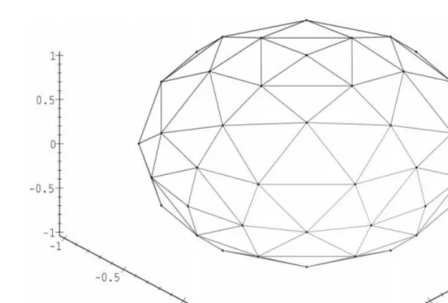
Fig. 1. 128 triangular patches approximating the unit sphere.
discretized. This will lead to a detailed analysis and numerical implementations in the following sections.
Assume that is approximated by piecewise planes h and the intersection of the half-spaces
bounded by these planes forms a polyhedron approximation of the obstacle domain− with all their vertices lying on . Assume that h consists of piecewise triangles parametrized by the maximum
side length, which is generically denoted by h, and assume that the aspect ratio of radii of circum-sribing circles and inscribed circles of all the individual triangle patches are bounded above and below as h approaches 0. It follows from analysis in the appendix that these triangulation meshes h
approximate in the order of h if is twice continously dierentiable. From this some important properties of the integral operator on are preserved on h, which is the key to the results which
follow. We will illustrate this in detail in the next section.
The N patches of the triangulated meshes are assumed to be numbered sequentially in some convenient way and the individual patch is denoted by n. The centroid and the diameter of nth
patch are denoted by xn and hn, respectively. We also denote the area of nth patch by sn. In C3N,
we introduce the inner product (·;·)W dened by
(u;C)W:=
N
X
n=1;n∈ h
(un;Cn)sn (3.1)
and denote the resulting inner product space by U and the associated norm by
||u||W:=
p
where in (3.1) (·;·) is the inner product in C3. The inner product and norm thus dened are associated with the discrete L2 inner product and norm on
h.
To discretize (2.15) on h, we approximate the surface current J(x) =n(x)×H(x) by piecewise
constant function ˜J, which takes a complex vector Jm in mth triangle patch, and evalute both sides of (2.15) at xk, k= 1; : : : ; N: The resulting collocation scheme is as follows
The linear system (3.3) has 3N unknowns and 3N equations. The following theorem shows that (3.3) is uniquely solvable provided (2.15) has a unique solution.
Theorem 3.1. Assume that (2.15) has a unique solution. Then for h small enough, there exists
c ¿0 such that
||1
2J+ ˜KJ||W¿c||J||W; (3.5)
where J is any vector in C3N.
Proof. Even though h is a piecewise linear boundary instead of twice continuously dierentiable,
Theorem 2.3 and (2.17) still hold if h is small. This follows from the approximation of h to .
For details, see the estimates in the appendix. So by (2.17) there exists c1¿0 such that
||(1
2I +K)J||L2( h)¿c1||J||L2( h); (3.6)
for any complex vector function J which is constant Jm in each triangle patch m. So
On kth patch k
By Theorem A.1 in the appendix, we have
|nk−nl||K(x;y)−K(xk;y)|6 L
where L depends on the curvature of and the aspect ratio of the meshes. A simple computation shows
lim
h→0(K(x;y)−K(xk;y)) = 0 a:e:x;y:
Collecting all these and applying dominant convergence theorem twice, we conclude that for any
¿0, there exists h1 such that when h ¡ h1 we have
if h is small enough.
The unique solvability of (3.3) now follows from Theorem 3.1, since the homogeneous system has only the trivial solution.
4. Error estimate
In this section an error estimate will be given for the collocation scheme (3.3). We will show that the error under the appropriate norm is of the rst order in the mesh size h.
First we introduce the error vector e∈C3N
where each ek∈C3 is dened on the kth triangle patch such that
ek:=Jk−J(xk): (4.2)
Next apply (2.15) on h and evalute both sides at xk:
1
By subtracting (4.3) from (3.3), we obtain
1
The main result in this section is the following theorem:
Theorem 4.1. Denote by J∈C3N the solution of (3.3)and byJ(x)∈(H1(
Proof. Let us rst estimate the right-hand side of (4.4):
The last step follows since J(y)−J(xl) is perpendicular to the unit normal nl of the lth patch. By
the estimates in the appendix, we obtain
|nk−nl||K(xk;y)|6 L
|xk−y|;
|nk·K(xk;y)|6 L
|xk−y|
;
where L depends on the curvature of and the aspect ratio of the triangular meshes h. Thus
|nk
Then by the Cauchy–Schwartz inequality,
A2
is a bounded function in y.
By a standard approximation result in nite element methods (see e.g., [2, 12, 13]), we obtain
Z
h
|J˜(y)|2ds
y6L4h2|J|2(H1(
h))3; (4.6)
where L4 depends only on the aspect ratio. Combining all these results yields
||1
2e+ ˜Ke||W6L5h 2|J|2
(H1(
h))3: (4.7)
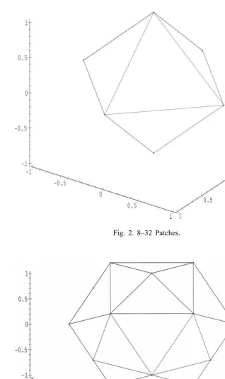
Fig. 2. 8–32 Patches.
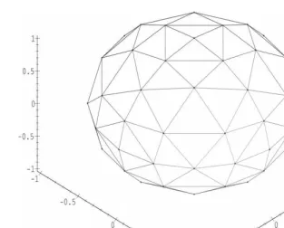
Fig. 4. 128–512 Patches.
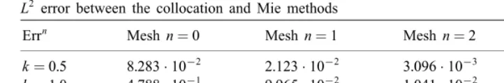
Table 1
L2 error between the collocation and Mie methods
Errn Meshn= 0 Meshn= 1 Mesh n= 2 Meshn= 3
In this section we describe the implementation and the numerical results of the collocation algo-rithm in previous sections for solving the surface currentn×H from the boundary integral equation (2.15).
We consider the electromagnetic scattering by a prefect conductor occupying an unit ball{(x; y; z) :
x2+y2+z261}. The incident wave propagates in the positive direction of z-axis:
where ˆx, ˆy are, respectively, unit vectors in the direction of x- and y-axis.
The resulting scattering eld can be computed by the Mie series which uses spherical harmonics and Bessel functions to represent the electromagnetic eld in an innite series, see [10, 11, 1]. The Mie series package by Warren J. Wiscombe (at ftp : ==emlib:jpl:nasa:gov=pub=miev:tar:Z) is used to compute the far-eld pattern of the magnetic eld. The far-eld pattern or the scattering amplitude H∞( ˆr) or H∞(; ) is dened on the unit sphere such that (see [3]) orthogonal to ˆr so that it can be decomposed into
H∞(; ) =H(; ) ˆ+H(; ) ˆ;
where ˆ, ˆ are two orthogonal unit vectors that are in the tangent plane of the unit sphere at ˆr. In this numerical experiment we will compare H and H obtained from the Mie series with those
from our collocation algorithm.
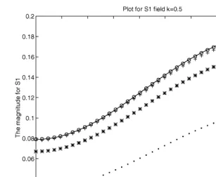
Fig. 6. Plot of|S1()| and |S2()|fork= 0:5
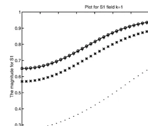
Fig. 8. Plot of |S1()|and |S2()|fork= 1.
Second-order quadrature rule is used to approximate the integrals and the Gauss–Seidel iterative scheme is used to solve the linear system (3.3) in order to save the memory load of storing the dense matrix. The surface current J(x) thus obtained is used to compute the scattering eld Hs(x)
Hs(x) =− 1
and the far-eld pattern H∞(; ) is then computed by using a second-order quadrature rule to approximate the following integral: The computatuions are performed on the triangular meshes corresponding to the rst four iterations of mesh renement in Figs. 2–5. In most literature S1() and S2() are computed where
on the triangular meshes corresponding to the iterationn=0; : : : ;3, respectively (see Figs. 2–5). Then the corresponding discrete L2 errors between the Mie series solution and the collocation schemes are dened by
The results in Table 1 show that the errors decrease in the average order O(h2) as the meshes get renement each time.
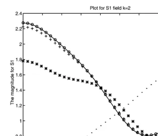
Figs. 6–11 are the corresponding plots of |Sn
m()| and |SmM()| for m= 1;2 and for n= 0; : : : ;3.
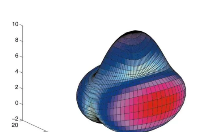
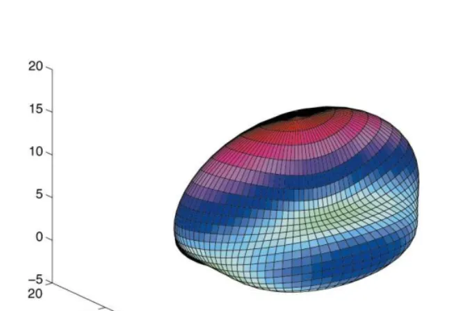
Here the solution by the Mie series is represented by the solid line, while the numerical solutions for n= 0 by the dot line, n= 1 by the star line, n= 2 by the plus line and n= 3 by the circle line. We also present here the three-dimensional radar cross section. We recall by denition that the bistatic radar cross section (; ) is dened by [1]
where Hs and Hi represent the scattered and incident magnetic eld, respectively. It can be shown [1] that, for an incident magnetic eld of unit magnetic eld, the bistatic radar cross section can also be represented by
(; ) =4
Fig. 10. Plot of|S1()|and |S2()| fork= 2.
Fig. 12. RCS plot of (; ) fork= 2 with n= 1;2.
Fig. 14. RCS plot of (; ) fork= 2 with n= 3 and Mie series.
Figs. 12–15 are the corresponding plots of (; ) fork= 2 when the iteration n= 1;2;3 are used.
Appendix
Since h is not twice continuously dierentiable, we may not directly use the results of [3] in
some estimates of previous sections. In this appendix we give the following two estimates that will be needed for our purpose.
Theorem A.1. Denote the centroid of the kth patch k by xk and y∈l. Then
|nk−nl|6C|xk−y|; (A.1)
|nk·(nk−y)|6C|xk−y|2; (A.2)
where the constant C depends on the curvature of and the aspect ratio of h. First the following
lemma is needed to prove (A.1) and (A.2)
Lemma A.2. In the triangular patch k
|nk−n(y)|6Chk; (A.3)
wheren(y) is the unit normal of aty and the projection ofy onto h is in k, hk is the diameter
of k.
The proof of (A.3) is a routine application of Taylor expansion and omitted here. The constant
C in (A.3) depends on the curvature of and the aspect ratio of k. To this end,we need the
following.
Denition. Dene the lifting operator L on h such that for any y∈l, we have Ly∈ and Ly−y⊥l.
The lifting operator L is well dened since is convex. By Taylor expansion we can show that if
y∈l
|Ly−y|6Chl; (A.4)
where C depends on the curvature of . Now we are in a position to prove Theorem A.1.
Proof of (A.1). First we claim that
|Lxk−Ly|6C|xk−y|: (A.5)
To verify (A.5), we see that (i) If |xk−y|61
3max(hk; hl), then
|Lxk−Ly|6|Lxk−xk|+|Ly−y|+|xk−y|
6|xk−y|+C(hk+hl) by (A:4)
(ii) If|xk−y|613hk, then bothxk andy are in thekth triangular patch andLis a Lipschitz operator
in k, so (A.5) follows.
Now from (A.5) and [3] we obtain
|nk−nl|6|nk−n(L(xk))|+|n(L(xk))−n(L(y))|+|n(L(y))−nl|
6C(hk+hl) +|L(xk−y)|
6C(hk+hl) +C1|xk−y|:
From this (A.1) follows.
Proof of (A.2). Since any point in a given triangular patch is the convex combination of its vertices, we can nd vertices x0 and y0 in the patch k and l, respectively, such that
|x0−y0|6C|xk−y| (A.6)
for y∈l and C62.
Since xk−x0⊥nk and y−y0⊥nl
|nk·(xk−y)|=|nk·(x0−y)|
6|(nk−nl)·(x0−y)|+|nl·(x0−y)|
6C|xk−y|2+|nl·(x0−y0)| (A:1)
6C|xk−y|+|nl−n(y0)||x0−y0|+|n(y0)·(x0−y0)|: Since x0, y0∈ ,
|n(y0)·(x0−y0)|6C1|x0−y0|2: (A.7)
Combining all these, we have
|nk·(xk−y)|6C(|xk−y|2+h
l|xk−y|):
Now after using a scale change argument among hk, hl and |xk−y|, we conclude
|nk·(xk−y)|6C|xk−y|2:
References
[1] J.J. Bowman, T.B.A. Senior, P.L.E. Uslenghi, Electromagnetic and Acoustic Scattering by Simple Shapes, North-Holland, Amsterdam, 1969.
[2] P.G. Ciarlet, The Finite Element Method for Elliptic Problems, North-Holland, Amsterdam, 1978. [3] D. Colton, R. Kress, Integral Equation Methods in Scattering Theory, Wiley, New York, 1983.
[4] M. Feistauer, G.C. Hsiao, R.E. Kleinman, Asymptotic and a posterior estimates for boundary element solutions of hypersingular integral equations. SIAM J. Numer. Anal. 33 (1996) 666–685.
[6] G.C. Hsiao, R.E. Kleinman, Error analysis in numerical solution of acoustic integral equations, Int. J. Numer. Meth. Eng. 37 (1994) 2921–2933.
[7] G.C. Hsiao, R.E. Kleinman, Error control in numerical solution of boundary integral equation, ACES 11 (1996) 32–36.
[8] G.C. Hsiao, R.E. Kleinman, Mathematical foundations for error estimation in numerical solutions of integral equations in electromagnetics, IEEE Trans Antennas Propagation 45 (1997) 316–328.
[9] G.C. Hsiao, R.E. Kleinman, R.X. Li, P.M. van den Berg, Residual error – a simple and sucient estimate of actual error in solutions of boundary integral equations, in S.Grilli, C.A. Brebbia, A.H. Cheng (Eds.), Computational Engineering with Boundary Eelments, vol. 1: Fluid and Potential Problems, Computational Mechanics Publication, Southampton, Boston, (1990) 73–83.
[10] H.C. van de Hulst, Light Scattering by Smaller Particles, Dover, New York, 1981.
[11] M. Kerker, The Scattering of Light and Other Electromagnetic Radiation, Academic Press, New York, 1969. [12] R.A. Nicolaides, D.-Q. Wang, Convergence analysis of a covolume scheme for Maxwell’s equations in three
dimensions, Math. Comput., to appear.
[13] R.A. Nicolaides, D.-Q. Wang, Convergence analysis of a covolume scheme for electromagnetic scattering in three dimensions, preprint, 1996.
[14] A.W. Maue, Zur Formuliering eins allgemenen Beugungsproblems durch eine integraleichung, Z. Phys. 126 (1949) 601–618.
[15] F.H. Murray, Conductors in an electromagnetic eld, Amer. J. Math. 53 (1931) 275–288.
[16] J.A. Stratton, L.J. Chu, Diraction theory of electromagnetic waves, Phys. Rev. 56 (1939) 99–107. [17] A.E. Taylor, Functional Analysis, Wiley, New York, 1958.