CHAPTER IV RESULT OF THE STUDY
This chapter covered description of the data, test of normality and
homogeneity, result of the data analysis and discussion. A. Description of The Data
In this section, it would be described the obtained data of the students’ vocabulary score after and before taught by using CTL. The
presented data consisted of Mean, Standard Deviation, Standar Error, and
the figure.
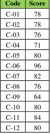
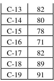
1. The Description of Pre-Test Score
The students’ score could be distributed by the following table in order to analyze the students’ mastery before conducting the treatment.
Table 4.1 The Description Data of Students’ Pre-Test Score
C-13 82 knowledge before conducting the treatment. To determine the frequency of score, percent of score, valid percent and cumulative
percent calculated using SPSS 18 as follows:
Table 4.2 The frequency of score, percent of score, valid percent andcumulative percent calculated using SPSS 18
The next step, the result calculated the scores of mean, standard deviation, and standard error using manual calculation as
follows:
1) Calculating Mean
Mx = =
= 79,89
2) Standard Deviation
S = √
S = √
S = √ = 7,063
3) Standard Error
SEmd =
√ = √ =
√ =
= 1,666
Based on the data above from the result of manual calculation, it was found that the mean score of pre-test was 79,89, the standard deviation was 7,063 and for the standard error was 1,666.
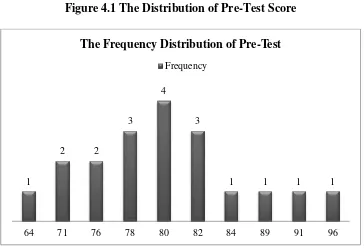
The distribution of students’ pre-test score can also be seen in
Figure 4.1 The Distribution of Pre-Test Score
It can be seen from the figure above the students’ pre-test
score. Therewas one student who got score 64. There were two students who got score 71. There were two students who got score 76. There were three students who got score 78. There were four students who got
score 80. There were three students who got score 82. There was one students who got score 84. There was one students who got score 89.
There was one students who got score 91. And there was one students who got score 96.
The next step, the result calculated the scores of mean,
standard deviation, and standard error using SPSS 18 program as follows:
1
2 2
3
4
3
1 1 1 1
64 71 76 78 80 82 84 89 91 96
Table 4.3 the Calculation of Mean, SD and SE using SPSS 18
Based on the table above, the result calculation using SPSS 18,
it was found that the mean of score pre-test was 79,89, the standard deviation 7,256 and the standard error of mean of the pre-test score was
1,665.
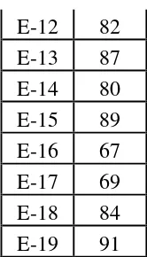
2. The Description of Post-Test Score
The students’ score could be distributed by the following table in order to analyze the students’ mastery after conducting the treatment.
E-12 82 knowledge before conducting the treatment. To determine the
frequency of score, percent of score, valid percent and cumulative percent calculated using SPSS 18 as follows:
Table 4.5 The frequency of score, percent of score, valid percent andcumulative percent calculated using SPSS 18
The next step, the result calculated the scores of mean, standard deviation, and standard error using manual calculation as
follows:
1) Calculating Mean
Mx = =
= 84,21
2) Standard Deviation
S = √
S = √
S = √ = 7,878
3) Standard Error
SEmd =
√ = √ =
√ =
= 1,858
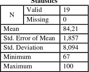
Based on the data above from the result of manual calculation, it was found that the mean score of post-test was 84,21, the standard deviation was 7,878 and for the standard error was 1,858.
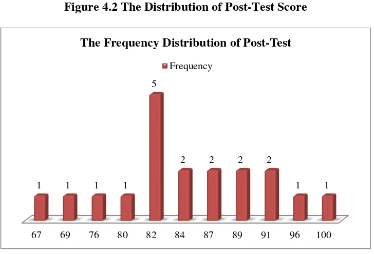
Figure 4.2 The Distribution of Post-Test Score
It can be seen from the figure above the students’ post-test
score. There was one student who got score 67. There was one students who got score 69. There was one students who got score 76. There was one students who got score 80. There were five students who got score
82. There were two students who got score 84. There were two students who got score 87. There were two students who got score 89. There
were two students who got score 91. There was one students who got score 96. And there was one students who got score 100.
The next step, the result calculated the scores of mean,
standard deviation, and standard error using SPSS 18 program as follows:
67 69 76 80 82 84 87 89 91 96 100
1 1 1 1
5
2 2 2 2
1 1
Table 4.6 the Calculation of Mean, SD and SE using SPSS 18
Based on the table above, the result calculation using SPSS 18,
it was found that the mean of score post-test was 84,21, the standard deviation 8,094 and the standard error of mean of the post-test score was 1,857.
B. Testing of Normality and Homogeneity 1. Normality Test
Itused to know the normality of the data that was going to be analyzed whether both groups have normal distribution or not. Because of that, the normality test used SPSS 21 to measure the normality of the
data.
Table 4.7 Testing Normality of Post-Test Using SPSS 18 Tests of Normality
Kelompok Kolmogorov-Smirnova Shapiro-Wilk
Statistic df Sig. Statistic df Sig.
Score Pre-test ,175 19 ,127 ,955 19 ,484
Post-test ,182 19 ,098 ,956 19 ,495
If respondent > 50 used Kolmogorov-Sminornov
The criteria of the normality test pre-test was if the value of (probability value/critical value) was higher than or equal to the level of
significance alpha defined (r > a), it meant that the distribution was normal. Based on the calculation using SPSS 18 above, the value of
(probably value/critical value) from post-test of class in Saphiro-Wilkv table was higher than level of significance alpha used or r = 0,495> 0,05. So, the distribution was normal. It meantthe students’ score of post-test had normal distribution.
2. Testing of Data Homogeneity
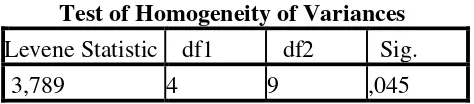
Table 4.8 Homogeneity Test Test of Homogeneity of Variances Levene Statistic df1 df2 Sig.
3,789 4 9 ,045
The criteria of the homogeneity post-test was if the value of (probability value/critical value) was higher than or equal to the level
significance alpha defined (r>a), it meantthe distribution was homogeneity. Based on the calculation using SPSS 18 program above,
the value of (probably value/critical value) from pre-test of experiment and control class on homogeneity of variance in sig column was known that p-value was 0,045 or 0,05. The data in this study fulfilled
C. The Result of Data Analysis
1. Testing hypothesis using Manual Calculation
The level of significance used 5%. It meant that the level of significance of the refusal null hypothesis in 5%. The level of
significance decided at 5% due to the hypothesis type stated on non-directional (two-tailed test). It meant that the hypothesis cannot directly the prediction of alternative hypothesis. To test the hypothesis of the
study used t-test statistical calculation. First, it calculated the mean and the standard deviationpost-test. It was found the standard deviation and
thestandard error of post-test at the previous data presentation. It could be seen in this following table:
Table 4.9 Mean and the Standard Deviation of Pos-Test
Group Mean Standard Deviation
Post-Test 84,21 7,878
The table showed the result of the mean calculation of post-test
group was 84,21 and the result of standard deviation was 7,878. To examine the hypothesis, the writer used the formula as follow:
To =
√ ⁄
=
√ ⁄
=
⁄
=
Which the criteria:
If t-test (t-observed) ≥ t-table, Ha was accepted and H0 was rejected If t-test (t-observed) ≤ t-table, Ha was rejected and H0 was accepted Then, the degree of freedom (df) accounted with the formula:
Df = (N – 1) = 19 – 1 = 18
The significant levels choose at 5%, it meant the significant level of refusal of null hypothesis at 5%. The significance level decided
at 5% to the hypothesis stated on non-directional (two-tailed test). It meant that the hypothesis cannot direct the prediction of alternative hypothesis. The calculation above showed the result of ttest calculation
as in the table follows:
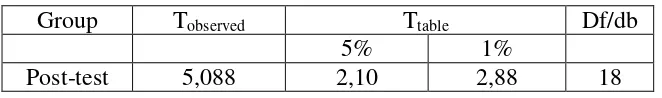
Table 4.10 the Result of ttestManual Calculation
Group Tobserved Ttable Df/db
5% 1%
Post-test 5,088 2,10 2,88 18
Based on the result of hypothesis test calculation, it was found that the value of tobserved was greater than the value of ttable at the level
significance in 5% or tobserved>ttable(5,088> 2,10). It meant Ha was accepted and H0 was rejected.
2. Interpretation
result of the degree of freedom (df) was 18, it found from total number of the students in group minus 1. The following table was the result of
tobserved and ttable from 18 df at 5% significance level.
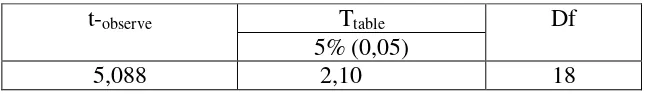
Table 4.11The Result of T-Test Using Manual Calculation
t-observe Ttable Df
5% (0,05)
5,088 2,10 18
The interpretation of the result of t-test using manual
calculation , it was found the t-observed was higher than t-table at 5% level or 5,088 > 2,10. It could be interpreted based on the result of calculation that Ha stating that there wasany significant effect of
contextual teaching and learning on vocabulary mastery at tenth graders of SMA Muhammadiyah Palangka Raya was accepted and H0 stating that there wasno effect of contextual teaching and learning on
vocabulary mastery at tenth graders of SMA Muhammadiyah Palangka Raya was rejected. It meant that teaching vocabulary by using
contextual teaching and learningthere was effect toward students’ vocabulary mastery.
D. Discussion
Meanwhile, after the data was calculated using ttest, it was found that the value of ttest was higher than ttable at 5% level of significancettest = 5,088 ttable= 2,10. This
finding indicated that the alternative hypothesis stating that there was significant effect of using contextual teaching and learning of the tenth grade students at
SMA Muhammadiyah 1 Palangka Raya was accepted. On the contrary, the null hypothesis stating that there was no any significant effect of using contextual teaching and learning of the tenth grade students at SMA Muhammadiyah 1
Palangka Raya was rejected.
Contextual Teaching and Learning was one of method used to teach
English vocabulary by the teacher for teaching the students in the class. Contextual Teaching and Learning made a good interaction between teacher and students. Contextual Teaching and Learning used by teacher increased students’ enthusiasm in learning process. The result of study is in line with the opinion Carr,M in chapter II page 27 As explain above, that CTL help us relate us subject matter content to real world situations and motivates to make connections between knowledge and its application to their personal, social, and cultural circumstances in their lives. Therefore, the strategies in using CTL techniques
are:62 It mean could be occurred because Contextual Teaching and Learning connected between material and the fact in real situation. From the result of
analysis, it could be seen from the score of students how the use of method giving positive effects for students vocabulary mastery. It meant the method has important role in teaching learning process.
62
The findings of the study verified the statement that teaching Vocabulary using Contextual Teaching and Leaning as a good method in
teaching English vocabulary that provided the concrete thing for the students that can be seen.The result of study is in line with the opinionClemente Charles
Hudsonin chapter II page 21. Contextual Teaching and Learning was a conception of teaching and learning that help teacher relate subject matter content to real word situations and motivates students’ to make connections
between knowledge, to their lives as family members, citizens, and workers, and engage in the hard work that learning requires.63 It proved by the calculation
result of the acceptance of alternative hypotheses stating that teaching vocabulary using Contextual Teaching and Learning gave effect toward the vocabulary mastery at the tenth grade students at SMA Muhammadiyah 1
Palangka Raya.
63 Clemente Charles Hudson, &Vesta R. Whisler, ‘Contextual Teaching and