(Supplemental Document)
Zhirong Yang1,2,3, Jaakko Peltonen1,3,4 and Samuel Kaski1,2,3 1Helsinki Institute for Information Technology HIIT, 2University of Helsinki,
3Aalto University,4University of Tampere
Abstract
This supplemental document provides addi-tional information that does not fit in the pa-per due to the space limit. Section 1 gives related mathematical basics, including ma-jorizations of convex and concave functions, as well as the definitions of information diver-gences. Section 2 presents more examples on developing MM algorithms for manifold em-bedding, in addition to the t-SNE included in the paper. Section 3 illustrates that many existing manifold embedding methods can be unified into the Neighbor Embedding frame-work given in Section 5 of the paper. Section 4 provides proofs of the theorems in the pa-per. Section 5 gives an example of QL be-yond manifold embedding. Section 6 gives the statistics and source of the experimented datasets. Section 7 provides supplemental experiment results.
1
Preliminaries
Here we provide two lemmas related to majorization of concave/convex functions and definitions of infor-mation divergences.
1.1 Majorization of concave/convex functions
1) A concave function can be upper-bounded by its tangent.
Appearing in Proceedings of the 18th
International Con-ference on Artificial Intelligence and Statistics (AISTATS) 2015, San Diego, CA, USA. JMLR: W&CP volume 38. Copyright 2015 by the authors.
Lemma 1. If f(z)is concave in z, then
For a scalar concave function f(), this simplifies to
f(˜x) ≤ G(˜x, x) = ˜xf′(x) + constant. Obviously, 2) A convex function can be upper-bounded by using the Jensen’s inequality.
Lemma 2. Iff(z)is convex inz, and˜x= [˜x1, . . . ,x˜n]
tives also match:
∂G(˜x, x) 1.2 Information divergences
D(p||q) = 0 iff p = q. To avoid notational clutter we only give vectorial definitions; it is straightforward to extend the formulae to matrices and higher-order tensors.
Let Dα, Dβ, Dγ, andDr respectively denote α-, β-,
γ-, and R´enyi-divergences. Their definitions are (see e.g. [3])
wherepiandqiare the entries inpandqrespectively, ˜
pi = pi/Pjpj, and ˜qi = qi/Pjqj. To handle p’s containing zero entries, we only consider nonnegative
α, β, γ and r. These families are rich as they cover most commonly used divergences in machine learning such as normalized Kullback-Leibler divergence (ob-tained fromDr with r→1 or Dγ with γ→1), non-normalized KL-divergence (α→1 orβ→1), Itakura-Saito divergence (β→0), squared Euclidean distance (β = 2), Hellinger distance (α= 0.5), and Chi-square divergence (α= 2). Different divergences have become widespread in different domains. For example,DKLis widely used for text documents (e.g. [7]) and DIS is popular for audio signals (e.g. [4]). In general, estima-tion using α-divergence is more exclusive with larger
α’s, and more inclusive with smallerα’s (e.g. [10]). For
β-divergence, the estimation becomes more robust but less efficient with larger β’s.
2
More Development Examples
The paper provides an example of developing a MM algorithm for t-Distributed Stochastic Neighbor Em-bedding (t-SNE); here we provide additional examples of developing MM algorithms for other manifold em-bedding methods.
2.1 Elastic Embedding (EE)
Given a symmetric and nonnegative matrixP andλ >
0, Elastic Embedding [2] minimizes
JEE(Ye) =
The EE objective is naturally decomposed into
A(P,Qe) =−X
The quadratification of A(P,Qe) is simply identical, withW =P. The final majorization function is
G(Y , Ye ) =X Thus the MM update rule of EE is
Ynew=LP+
2.2 Stochastic Neighbor Embedding (SNE)
Suppose the input matrix is row-stochastic, i.e.Pij ≥0 and PjPij = 1. Denote ˜qij = exp −ky˜i−y˜jk2and
e
Qij = ˜qij/Pbq˜ib. Stochastic Neighbor Embedding [6] minimizes total Kullback-Leibler (KL) divergence betweenP andQe rows:
Thus we can decompose the SNE objective into
Again the quadratification of A(P,q˜) is simply iden-tical, with W = P. The final majorization function is
Thus the MM update rule of SNE is
Ynew =LP+PT +
Similarly, we can develop the rule for symmetric SNE (s-SNE) [12]:
; and for Neighbor Retrieval Visu-alizer (NeRV) [13]:
JNeRV(Y) =λ
where P and Qare defined same manner as in SNE, and
Suppose a weighted undirected graph is encoded in a symmetric and nonnegative matrix P (i.e. the weighted adjacency matrix). The node-repulsive Lin-Log graph layout method [11] minimizes the following energy function:
Since the square root function is concave, by Lemma 1 we can upper boundA(P,Qe) by cation phase. The final majorization function of the LinLog objective is
G(Y , Ye ) =X
where ◦ is the elementwise product. Then the MM update rule of LinLog is
Ynew=LP◦Q+ρ
2.4 Multidimensional Scaling with Kernel Strain (MDS-KS)
Strain-based multidimensional scaling maximizes the cosine between the inner products in the input and output spaces (see e.g. [1]):
JMDS-S(Ye) = and simply lead to kernel PCA of P. In this exam-ple we instead consider a nonlinear embedding kernel
e
Qij = exp(−ky˜i−y˜jk2), where the corresponding ob-jective function is
P
and maximizing it is equivalent to minimizing its neg-ative logarithm We decompose the MDS-KS objective function into
We can upper boundA(P,Qe) by the Jensen’s inequal-ity (Lemma 2):
A(P,Qe)≤ −X
abPabQab in the quadratification
phase.
The final majorization function of the MDS-KS objec-tive is
3
Neighbor Embedding
In Section 5 of the paper, we review a framework for manifold embedding which is called Neighbor Embed-ding (NE) [16, 17]. Here we demonstrate that many manifold embedding objectives, including the above examples, can be equivalently formulated as an NE problem.
NE minimizesD(P||Qe), whereDis a divergence from
α-, β-, γ-, or R´enyi-divergence families, and the em-bedding kernel in the paper is parameterized asQeij =
c+aky˜i−y˜jk2
−b/a
for a ≥ 0, b > 0, and c ≥ 0 (adapted from [15]).
First we show the parameterized form of Qe includes the most popularly used embedding kernels. When
a = 1, b = 1, and c = 1, Qeij = 1 +ky˜i−y˜jk2
−1
is the Cauchy kernel (i.e. the Student-t kernel with a single degree of freedom); when a → 0 and b = 1,
e
Qij = exp −ky˜i−y˜jk2is the Gaussian kernel; when
a= 1, b= 1/2,c= 0,Qeij =ky˜i−y˜jk−1 is the inverse to the Euclidean distance.
Next we show some other existing manifold embed-ding objectives can equivalently expressed as NE. Ob-viously SNE and its variants belong to NE. Moreover, we have
4.1 Proof of Theorem 1
Proof. SinceB is upper-bounded by its Lipschitz sur-rogate
B(P,Qe) =B(Ye)≤B(Y) +hΨ,Ye−Yi+ρ
2kYe −Yk
2
F, we have H(Y, Y) = G(Y, Y). Therefore J(Y) =
H(Y, Y) = G(Y, Y)≥G(Ynew, Y)≥ J(Ynew), where
the first inequality comes from minimization and the second is ensured by the backtracking.
4.2 Proof of Theorem 2
The proposed MM updates share many convergence properties with the Expectation-Maximization (EM) algorithm. In this section we follow the steps in [14] to show that the MM updates will converge a stationary point ofJ. A stationary point can be a local optimum or a saddle point.
The convergence result is a special case of the Global Convergence Theorem (GCT; [19]) which is quoted be-low. A map A from points of X to subsets of X is called a point-to-set map on X. It is said to be closed atxifxk→x,xk∈Xandyk→y,yk∈ A(xk), imply
y ∈ A(x). For point-to-point map, continuity implies closedness.
Global Convergence Theorem. (GCT; from [14]) Let the sequence {xk}∞k=0 be generated by xk+1 ∈
M(xk), where M is a point-to-set map on X. Let a solution set Γ∈X be given, and suppose that:
i all points xk are contained in a compact set S ⊂
X;
ii M is closed over the complement ofΓ;
iii there is a continuous function αonX such that
(a) if x /∈Γ,α(x)> α(y)for ally∈ M(x), and (b) ifx∈Γ,α(x)≥α(y)for ally∈ M(x)
Then all the limit points of {xk} are in the solution set Γ and α(xk) converges monotonically to α(x) for some x∈Γ.
The proof can be found in [19].
Before showing the convergence of MM, we need the following Lemmas. For brevity, denoteM:Y →Ynew
the map by using the MM update Eq. 4 in the paper. LetS and F be the sets of stationary points of J(Y) and fixed points of M, respectively.
Lemma 3. S=F.
Proof. The fixed points of the MM update rule appear when
Y = (2LW+WT +ρI)−1(−Ψ +ρY)
(2LW+WT +ρI)Y = (−Ψ +ρY)
2LW+WTY + Ψ =0, (1)
which is recognized as ∂∂HYe
e
Y=Y = 0. Since we re-quire the majorization function Hshares the tangent with J, i.e. ∂∂JYe
e
Y=Y = ∂H
∂Ye
Ye=Y, Eq. 1 is equivalent to ∂∂JYe
e
Y=Y = 0, the condition of stationary points of J. ThereforeF ⊆S.
On the other hand, because QL requires that Gand J share the same tangent atY, and thus ∂∂JYe
e
Y=Y = 0 implies ∂∂YGe
e
Y=Y = 0, i.e. Y =M(Y). TherforeS ⊆
F
Lemma 4. J(Ynew)<J(Y)ifY /∈F.
Proof. Because G is convexly quadratic, it has a unique minimum Ynew =M(Y). IfY /∈ F, i.e.Y 6=
M(Y), we haveY 6=Ynew, which implies J(Ynew)≤ G(Ynew, Y)< G(Y, Y) =J(Y).
Now we are ready to prove the convergence to station-ary points (Theorem 2).
Proof. Consider S the solution set Γ, and J the con-tinuous function α in the GCT theorem. Lemma 3 shows that this is equivalent to considering F the so-lution set. Next we show that the QL-majorization and its resulting map M fulfill the conditions of the GCT theorem: J(Ynew) ≥ J(Y) and the
bounded-ness assumption ofJ imply Condition i;Mis a point-to-point map and thus the continuity of Gover both
e
Y and Y implies the closedness condition ii; Lemma 4 implies iii(a); Theorem 1 in the paper implies iii(b). Therefore, the proposed MM updates are a special case of GCT and thus converge to a stationary point of J.
4.3 Proof of Theorem 3
Proof. Since Aij is concave to ky˜i −y˜jk2, it can be upper-bounded by its tangent:
Aij(Pij,Qeij) ≤Aij(Pij, Qij)
+
∂Aij
∂ky˜i−y˜jk2
e
Y=Y,ky˜i−y˜jk
2− ky
i−yjk2
=
∂A
ij
∂ky˜i−y˜jk2
e
Y=Y,ky˜i−y˜jk
That is,Wij =∂ky˜∂Ai−ij˜yjk2 4.4 Proof of Theorem 4
Proof. Obviously all α- and β-divergences are addi-tively separable. Next we show the concavity in the given range. Denoteξij=ky˜i−y˜jk2 for brevity.
α-divergence. We decompose an α-divergence into
Dα(P||Qe) =A(P,Qe) +B(P,Qe) + constant, where
The second derivative of
Aij = 1
β-divergence. We decompose a β-divergence into
Dβ(P||Qe) =A(P,Qe) +B(P,Qe) + constant, where
The second derivative of Aij =
P
ijlnQeij+ constant. We write
A(P,Qe) =X ij
Aij(Pij,Qeij) =
X
ij
PijQe−ij1
=X ij
Pij(c+aξij)b/a
B(P,Qe) =X ij
lnQeij.
The second derivative of Aij = Pij(c+aξij)b/a with respect toξij is (b−a)bPij(aξij+c)
b
a−2, which is
non-positive iff a≥b, or equivalently 0∈[1−a/b,∞].
4.5 Proof of Theorem 5
The proofs are done by zeroing the derivative of the right hand side with respect toλ(see [17]). The closed-form solutions of λ at the current estimate for τ ≥0 are
λ∗= arg min
λ Dα→τ(P||λQ) =
P
ijPijτQ1ij−τ
P
ijQij
!1
τ
,
λ∗= arg min
λ Dβ→τ(P||λQ) =
P
ijPijQτij−1
P
ijQτij
,
with the special case
λ∗= exp −
P
ijQijln(Qij/Pij)
P
ijQij
!
forα→0.
5
Examples of QL beyond Manifold
Embedding
To avoid vagueness we defined the scope to be manifold embedding, which already is a broad field and one of listed AISTATS research areas. Within this scope the work is general.
It is also naturally applicable to any other optimiza-tion problems amenable to QL majorizaoptimiza-tion. QL is applicable to any cost function J = A+B, where
A can be tightly and quadratically upper bounded by Eq. 2 in the paper, andB is smooth. Next we give an example beyond visualization and discuss its potential extensions.
Consider a semi-supervised problem: given a training set comprising a supervised subset {(xi, yi)}ni=1 and
an unsupervised subset{xi}Ni=n+1, wherexi∈RDare vectorial primary data andyi∈ {−1,1}are supervised labels, the task is to learn a linear functionz=hw, xi+
b for predictingy.
In this example a composite cost function is used:
J(w, b) =A(w, b) +B(w, b)
whereA(w) is a locality preserving regularizer (see e.g. [5])
A(w, b) =λ
N
X
i=1
N
X
j=1
Sij(zi−zj)2
andB(w, b) is an empirical loss function [9]
B(w, b) = (1−λ) n
X
i=1
[1−tanh(yizi)]
withλ∈[0,1] the tradeoff parameter andSijthe local similarity betweenxi andxj (e.g. a Gaussian kernel). Because B is non-convex and non-concave, conven-tional majorization techniques that require convex-ity/concavity such as CCCP [18] are not applicable. However, we can apply QL here (Lipschitzation to B
and quadratification toA), which gives the update rule forw(denoteX = [x1. . . xN]):
wnew=λXLS+ST
2
XT +ρI−1
∂B ∂w +ρw
.
This example can be further extended with the same spirit, where B is replaced by another smooth loss function which is non-convex and non-concave, e.g. [8]
B(w, b) = (1−λ) n
X
i=1
1− 1
1 + exp(−yizi)
2 ,
and XLS+ST
2
XT can be replaced by other positive semi-definite matrices.
6
Datasets
Twelve datasets have been used in our experiments. Their statistics and sources are given in Table 1. Below are brief descriptions of the datasets.
• SCOTLAND: It lists the (136) multiple directors of the 108 largest joint stock companies in Scotland in 1904-5: 64 non-financial firms, 8 banks, 14 in-surance companies, and 22 investment and prop-erty companies (Scotland.net).
• COIL20: the COIL-20 dataset from Columbia University Image Library, images of toys from dif-ferent angles, each image of size 128×128.
Table 1: Dataset statistics and sources
Dataset #samples #classes Domain Source
SCOTLAND 108 8 network PAJEK
COIL20 1440 20 image COIL
7SECTORS 4556 7 text CMUTE
RCV1 9625 4 text RCV1
PENDIGITS 10992 10 image UCI
MAGIC 19020 2 telescope UCI
20NEWS 19938 20 text 20NEWS
LETTERS 20000 26 image UCI
SHUTTLE 58000 7 aerospace UCI
MNIST 70000 10 image MNIST
SEISMIC 98528 3 sensor LIBSVM
MINIBOONE 130064 2 physics UCI
PAJEK http://vlado.fmf.uni-lj.si/pub/networks/data/ UCI http://archive.ics.uci.edu/ml/
COIL http://www.cs.columbia.edu/CAVE/software/softlib/coil-20.php CMUTE http://www.cs.cmu.edu/~TextLearning/datasets.html
RCV1 http://www.ai.mit.edu/projects/jmlr/papers/volume5/lewis04a/ 20NEWS http://people.csail.mit.edu/jrennie/20Newsgroups/
MNIST http://yann.lecun.com/exdb/mnist/
LIBSVM http://www.csie.ntu.edu.tw/~cjlin/libsvmtools/datasets/
• RCV1: text documents from four classes, with 29992 words.
• PENDIGITS: the UCI pen-based recognition of handwritten digits dataset, originally with 16 di-mensions.
• MAGIC: the UCIMAGIC Gamma Telescope Data Set, 11 numerical features.
• 20NEWS: text documents from 20 newsgroups; 10,000 words with maximum information gain are preserved.
• LETTERS: the UCILetter Recognition Data Set, 16 numerical features.
• SHUTTLE: the UCI Statlog (Shuttle) Data Set, 9 numerical features. The classes are imbalanced. Approximately 80% of the data belongs to class 1.
• MNIST: handwritten digit images, each of size 28× 28.
• SEISMIC: the LIBSVM SensIT Vehicle (seismic) data, with 50 numerical features (the seismic sig-nals) from the sensors on vehicles.
• MINIBOONE: the UCI MiniBooNE particle identi-fication Data Set, 50 numerical features. This dataset is taken from the MiniBooNE experiment
and is used to distinguish electron neutrinos (sig-nal) from muon neutrinos (background).
7
Supplemental experiment results
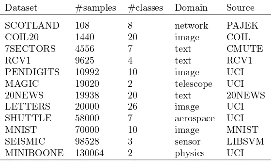
7.1 Evolution curves: objective vs. iteration
Figure 1 shows the evolution curves of the t-SNE ob-jective (cost function value) as a function of iteration for the compared algorithms. This supplements the results in the paper of objective vs. running time.
7.2 Average number of MM trials
The proposed backtracking algorithm for MM involves an inner loop for searching forρ. We have recorded the numbers of trials in each outer loop iteration. The av-erage number of trials is then calculated. The means and standard deviations across multiple runs are re-ported in Table 2.
We can see that for all datasets, the average number of trials is around two. The number is generally and slightly decreased with larger datasets. Two trials in an iteration means thatρremains unchanged after the inner loop. This indicates potential speedups may be achieved in future work by keepingρconstant in most iterations.
func-Figure 1: Evolution of the t-SNE objective (cost function value) as a function of iteration for the compared algo-rithms. The first and second rows were exactly calculated, while the third row uses Barnes-Hut approximation.
Table 2: Average number of MM trials and SD func-tion calls over all iterafunc-tions (mean ±standard devia-tion over 10 runs)
dataname N MM trials SD fun.calls SCOTLAND 108 2.00±0.00 21.91±1.88
COIL20 1.4K 1.94±0.11 1.92±0.29 7SECTORS 4.6K 2.00±0.00 3.06±0.34 RCV1 9.6K 2.00±0.00 2.56±0.09 PENDIGITS 11K 2.00±0.00 6.30±5.51 MAGIC 19K 2.00±0.00 2.12±0.06 20NEWS 20K 2.00±0.00 3.85±0.33 LETTERS 20K 2.00±0.01 13.30±4.00 SHUTTLE 58K 2.07±0.02 4.16±0.66
MNIST 70K 2.10±0.04 2.90±0.23 SEISMIC 99K 2.02±0.00 3.64±0.42 MINIBOONE 130K 2.07±0.01 3.29±0.20
tion calls to t-SNE objectives by the SD algorithm (last column of Table 2). It can be seen that the SD often requires more cost function calls than MM, which is one of the reasons that SD is slower.
7.3 ρvalue and number of MM trials vs. iteration
However, the above average number of trials does not mean that ρ will remain nearly constant around its initial value. Actually ρ can vary greatly in different iterations. See Figure 2 for example, where the ranges of ρ in the first 300 iterations are [3.6×10−21,2.6×
10−4], [6.2×10−8,1.6×10−5], and [3.9×10−9,4.0×
10−6] forCOIL20, 20NEWS, andMNIST, respectively.
References
[1] A. Buja, D. Swayne, M. Littman, N. Dean, H. Hofmann, and L. Chen. Data visualization with multidimensional scaling. Journal of Com-putational and Graphical Statistics, pages 444– 472, 2008.
[2] M. Carreira-Perpi˜n´an. The elastic embedding al-gorithm for dimensionality reduction. In ICML, pages 167–174, 2010.
[3] A. Cichocki, S. Cruces, and S.-I. Amari. General-ized alpha-beta divergences and their application to robust nonnegative matrix factorization. En-tropy, 13:134–170, 2011.
Itakura-Figure 2: Backtracking behavior statistics of MM for t-SNE: (left)ρvalues vs. iteration, and (right) number of trials in the backtracking algorithm. We only show the first 50 iterations for better visibility.
Saito divergence with application to music analy-sis. Neural Computation, 21(3):793–830, 2009.
[5] X. He, S. Yan, Y. Hu, P. Niyogi, and H. Zhang. Face recognition using laplacianfaces. IEEE Transactions on Pattern Analysis and Machine Intelligence, 27(3):328–340, 2005.
[6] G. Hinton and S. Roweis. Stochastic neighbor embedding. InNIPS, pages 833–840, 2002.
[7] T. Hofmann. Probabilistic latent semantic index-ing. In SIGIR, pages 50–57, 1999.
[8] F. Li and Y. Yang. A loss function analysis for classification methods in text categorization. In ICML, pages 472–479, 2003.
[9] L. Mason, J. Baxter, P. Bartlett, and M. Frean. Boosting algorithms as gradient descent in func-tion space. InNIPS, pages 512–518, 1999.
[10] T. Minka. Divergence measures and message pass-ing. Technical report, Microsoft Research, 2005.
[11] A. Noack. Energy models for graph clustering. Journal of Graph Algorithms and Applications, 11(2):453–480, 2007.
[12] L. van der Maaten and G. Hinton. Visualizing data using t-SNE. Journal of Machine Learning Research, 9:2579–2605, 2008.
[13] J. Venna, J. Peltonen, K. Nybo, H. Aidos, and S. Kaski. Information retrieval perspective to nonlinear dimensionality reduction for data visu-alization. Journal of Machine Learning Research, 11:451–490, 2010.
[14] J. Wu. On the convergence properties of the em algorithm.The Annals of Statistics, 11(1):95–103, 1983.
[15] Z. Yang, I. King, Z. Xu, and E. Oja. Heavy-tailed symmetric stochastic neighbor embedding. InNIPS, pages 2169–2177, 2009.
[16] Z. Yang, J. Peltonen, and S. Kaski. Scalable opti-mization of neighbor embedding for visualization. InICML, pages 127–135, 2013.
[17] Z. Yang, J. Peltonen, and S. Kaski. Optimization equivalence of divergences improves neighbor em-bedding. InICML, 2014.
[18] A. Yuille and A. Rangarajan. The concave-convex procedure. Neural Computation, 15:915– 936, 2003.