Maximum Likelihood Programming in R
Marco R. Steenbergen
Department of Political Science University of North Carolina, Chapel HillJanuary 2006
Contents
1 Introduction 2
2 Syntactic Structure 2
2.1 Declaring the Log-Likelihood Function . . . 2 2.2 Optimizing the Log-Likelihood . . . 4
3 Output 5
4 Obtaining Standard Errors 5
5 Test Statistics and Output Control 7
1
Introduction
The programming language R is rapidly gaining ground among political method-ologists. A major reason is that R is a flexible and versatile language, which makes it easy to program new routines. In addition, R algorithms are generally very precise.
R is well-suited for programming your own maximum likelihood routines. Indeed, there are several procedures for optimizing likelihood functions. Here I shall focus on theoptimcommand, which implements the BFGS and L-BFGS-B algorithms, among others.1
Optimization throughoptim is relatively straight-forward, since it is usually not necessary to provide analytic first and second derivatives. The command is also flexible, as likelihood functions can be de-clared in general terms instead of being defined in terms of a specific data set.
2
Syntactic Structure
Estimating likelihood functions entails a two-step process. First, one declares the log-likelihood function, which is done in general terms. Then one optimizes the log-likelihood function, which is done in terms of a particular data set. The log-likelihood function and optimization command may be typed interactively into the R command window or they may be contained in a text file. I would recommend saving log-likelihood functions into a text file, especially if you plan on using them frequently.
2.1
Declaring the Log-Likelihood Function
The log-likelihood function is declared as an Rfunction. In R, functions take at least two arguments. First, they require a vector of parameters. Second, they require at least one data object. Note that other arguments can be added to this if they are necessary. The data object is a generic placeholder for data. In theoptim command, specific data are substituted for this placeholder.
After the arguments are declared, the actual log-likelihood is expressed and demarcated by{}. Thus, we have the following syntax:
name<-function(pars,object){ declarations
logl<-loglikelihood function return(-logl)
}
Here name is the name of the log-likelihood function, pars is the name of the parameter vector, andobjectis the name of the generic data object. The in-structions placed between brackets define the log-likelihood function. At a mini-mum, there should be two elements here: (1) the declaration of the log-likelihood
1
Theoptimcommand also includes Nelder-Mead, conjugate gradients, and simulated an-nealing algorithms. Other optimization routines include optimize, nlm, and constrOptim. These procedures are not discussed here.
function, which is namedlogl, and (2) the return of negative one times the log-likelihood.2
In addition, it may be necessary to make other declarations. These may include partitioning a parameter vector or declaring temporary vari-ables that figure in the log-likelihood function. The application of this syntax will be clarified using several examples.
Example 1: Consider the Poisson log-likelihood function, which is given by
l=X
Since the last term does not include the parameter,µ, it can be safely ignored. Thus, the kernel of the log-likelihood function is
l=X
i
yiln(µ)−nµ
We can program this function using the following syntax: poisson.lik<-function(mu,y){
n<-nrow(y)
logl<-sum(y)*log(mu)-n*mu return(-logl)
}
Herepoisson.likis the name of the log-likelihood function; this name will be used in the optim command. The “vector” of parameters is called mu; this is not really a vector since there is only one parameter that needs to be estimated. Further, y is the placeholder for the data. Since the log-likelihood function requires knowledge of the sample size, we obtain this using n<-nrow(y). The expression forlogl contains the kernel of the log-likelihood function. Finally, we ask R to return -1 times the log-likelihood function.
Example 2: Imagine that we have a sample that was drawn from a normal distribution with unknown mean, µ, and variance, σ2
. The objective is to estimate these parameters. The normal log-likelihood function is given by
l = −.5nln(2π)−.5nln(σ2
We can program this function in the following way: normal.lik1<-function(theta,y){
mu<-theta[1] sigma2<-theta[2] n<-nrow(y)
2
We ask for−1×lbecause theoptimcommand minimizes a function by default. Mini-mization of−lis the same as maximization ofl, which is what we want.
logl< .5*n*log(2*pi) .5*n*log(sigma2) -(1/(2*sigma2))*sum((y-mu)**2)
return(-logl) }
Herethetais a vector containing the two parameters of interest. We declare the elements of this vector in the first two lines of the bracketed part of the program. Specifically, the first element (theta[1]) is equal toµ, while the second element (theta[2]) is equal toσ2
. The remainder of the program sets the sample size, specifies the log-likelihood function, and asks R to return the negative of this function.
Note that the normal log-likelihood function may also be written as
l = −nln(σ) +X
logl<- -n*log(sigma) - sum(log(dnorm(z))) return(-logl)
}
wherednormis R’s standard normal density function. Here we estimateσrather thanσ2
, but it is easy to move back and forth between these parameterizations.
2.2
Optimizing the Log-Likelihood
Once the log-likelihood function has been declared, then theoptim command can be invoked. The minimal specification of this command is
optim(starting values, log-likelihood, data)
Here starting values is a vector of starting values, log-likelihood is the name of the log-likelihood function that you seek to maximize, and data de-clares the data for the estimation. This specification causes R to use the Nelder-Mead algorithm. If you want to use the BFGS algorithm you should include the method="BFGS" option. For the L-BFGS-B algorithm you should declare method="L-BFGS-B". The current specification does not produce standard er-rors. A procedure for obtaining standard errors will be discussed later in this report.3
3
There are many other options for theoptimcommand. For a detailed description see, for example,http://jsekhon.fas.harvard.edu/stats/html/optim.html.
Example 3: Imagine that we have a vectordatathat consists of draws from a Poisson distribution with unknownµ. We seek to estimate this parameter and have already declared the log-likelihood function aspoisson.lik. Estimation using the BFGS algorithm now commences as follows
optim(1,poisson.lik,y=data,method="BFGS")
Here 1 is the starting value for the algorithm. Since the log-likelihood function refers to generic data objects asy, it is important that the vectordatais equated withy.
Example 4: Given a vector of data,y, the parameters of the normal distrib-ution can be estimated using
optim(c(0,1),normal.lik1,y=y,method="BFGS")
This is similar to Example 3 with the exception of the starting values. Since the normal distribution contains two parameters, two starting values need to be declared. Here we set the starting value for ˆµto 0 and the starting value for ˆσ2
to 1. These two values are “bundled” using thecor concatenation operator.
3
Output
Theoptim specifications discussed so far will produce several pieces of output. These come under various headings:
1. $par: This shows the MLEs of the parameters.
2. $value: This shows the value of the log-likelihood function at the MLEs. If you asked R to return -1 times the log-likelihood function, then this is the value reported here.
3. $counts: A vector that reports the number of calls to the log-likelihood function and the gradient.
4. $convergence: A value of 0 indicates normal convergence. If you see a 1 reported, this means that the iteration limit was exceeded. This limit is set to 10000 by default.
5. $message: This shows warnings of any problems that occurred during optimization. Ideally, one would like to seeNULLhere, since this indicates that there are no warnings.
4
Obtaining Standard Errors
Theoptim command allows one to compute standard errors based on the ob-served Fisher information matrix.4
This requires that we obtain the Hessian
4
Unlike Stata, standard errors, test statistics, and confidence intervals are not computed by default in theoptimcommand.
matrix, which can be done by addinghessian=Torhessian=TRUEto the com-mand. Since we will have to perform operations on the Hessian, it is also important that we store the results from the estimation into an object. The following linear regression example illustrates how to do this.
Example 5: Imagine that we are interested in estimating a simple linear regression for some simulated data. First, we create the data matrix for the predictors
X<-cbin(1,runif(100))
Here we draw 100 observations from a uniform distribution with limits 0 and 1. These data are bound together with the constant (1). Next, we postulate a set of values for the true parameters:
theta.true<-c(2,3,1)
Here, the first element is β0, the second element isβ1, and the last element is
σ2
. We can now create the dependent variable: y<-X%*%theta.true[1:2] + rnorm(100)
where rnorm(100) generates the disturbance by drawing 100 values from the standard normal distribution. We now have the data on the dependent variable and predictor.
The next step is to declare the log-likelihood function. The following syntax shows one way to do this.
ols.lf<-function(theta,y,X){
Herethetacontains both the elements ofβandσ2
. The program declares the firstkelements of thetato beβand thek+ 1st element to beσ2
. The vector econtains the residuals and t(e)%*%ein the log-likelihood function causes R to compute the sum of squared residuals.
We can now start the optimization of the log-likelihood function and store the results in an object namedp(any other name would have worked just as well):
p<-optim(c(1,1,1),ols.lf,method="BFGS",hessian=T,y=y,X=X)
wherec(1,1,1)sets the starting values for ˆβ0, ˆβ1, and ˆσ 2
equal to 1. We can now invert the Hessian to obtain the observed Fisher information matrix.5
This Hessian is stored asp$hessianand it can be inverted using
OI<-solve(p$hessian)
The square root of the diagonal elements are then the standard errors, corre-sponding to ˆβ0, ˆβ1, and ˆσ2, respectively. These can be obtained by typing
se<-sqrt(diag(OI))
5
Test Statistics and Output Control
With the standard errors in hand, Wald test statistics and their associated p -values can be computed. The following syntax will accomplish this task for the regression model of Example 5.
Example 5 Cont’d: The Wald test statistic is given by the ratio of the estimates and their standard errors. The associatedp-value can be computed by referring to a Student’s t-distribution with degrees of freedom equal to the number of rows minus the number of columns inX.
t<-p$par/se
pval<-2*(1-pt(abs(t),nrow(X)-ncol(X))) results<-cbind(p$par,se,t,pval)
results(colnames)<-c("b","se","t","p") results(rownames)<-c("Const","X1","Sigma2") print(results,digits=3)
The first line generates the test statistics, the second line computes the asso-ciated p-values, while the third line brings together the estimates, estimated standard errors, test statistics, and p-values. The fourth line creates a set of column headers for the output, while the fifth line creates a set of row headers. Finally, the last line causes R to print the results to the screen, with a precision of 3 digits.
5
The observed Fisher information is equal to (−H)−1. The reason that we do not have to
multiply the Hessian by -1 is that all of the evaluation has been done in terms of -1 times the log-likelihood. This means that the Hessian that is produced byoptimis already multiplied by -1.
Example of MLE Computations, using R
First of all, do you really need R to compute the MLE? Please note that
MLE in many cases have explicit formula. Second of all, for some common
distributions even though there are no explicit formula, there are standard
(existing) routines that can compute MLE. Example of this catergory include
Weibull distribution with both scale and shape parameters, logistic
regres-sion, etc. If you still cannot find anything usable then the following notes
may be useful.
We start with a simple example so that we can cross check the result.
Suppose the observations
X
1, X
2, ..., X
nare from
N
(
µ, σ
2
) distribution (2
parameters:
µ
and
σ
2).
The log likelihood function is
X
−
(
X
i−
µ
)
2
2
σ
2−
1
/
2 log 2
π
−
1
/
2 log
σ
2+ log
dX
i(actually we do not have to keep the terms
−1
/
2 log 2
π
and log
dX
isince
they are constants.
In R software we first store the data in a vector called
xvec
xvec <- c(2,5,3,7,-3,-2,0)
# or some other numbers
then define a function (which is negative of the log lik)
fn <- function(theta) {
sum ( 0.5*(xvec - theta[1])^2/theta[2] + 0.5* log(theta[2]) )
}
where there are two parameters:
theta[1]
and
theta[2]
. They are
compo-nents of a vector
theta
. then we try to find the max (actually the min of
negative log lik)
nlm(fn, theta <- c(0,1), hessian=TRUE)
or
You may need to try several starting values (here we used
c(0,1)
) for
the
theta
. ( i.e.
theta[1]=0, theta[2]=1
. )
Actual R output session:
> xvec <- c(2,5,3,7,-3,-2,0)
# you may try other values
> fn
# I have pre-defined fn
function(theta) {
sum( 0.5*(xvec-theta[1])^2/theta[2] + 0.5* log(theta[2]) )
}
> nlm(fn, theta <- c(0,2), hessian=TRUE)
# minimization
$minimum
[1] 12.00132
$estimate
[1]
1.714284 11.346933
$gradient
[1] -3.709628e-07 -5.166134e-09
$hessian
[,1]
[,2]
[1,]
6.169069e-01 -4.566031e-06
[2,] -4.566031e-06
2.717301e-02
$code
[1] 1
$iterations
[1] 12
> mean(xvec)
[1] 1.714286
# this checks out with estimate[1]
> sum( (xvec -mean(xvec))^2 )/7
[1] 11.34694
# this also checks out w/ estimate[2]
> output1 <- nlm(fn, theta <- c(2,10), hessian=TRUE)
> solve(output1$hessian)
# to compute the inverse of hessian
[,1]
[,2]
[1,] 1.6209919201 3.028906e-04
[2,] 0.0003028906 3.680137e+01
> sqrt( diag(solve(output1$hessian)) )
[1] 1.273182 6.066413
> 11.34694/7
[1] 1.620991
> sqrt(11.34694/7)
[1] 1.273182
# st. dev. of mean checks out
> optim( theta <- c(2,9), fn, hessian=TRUE)
# minimization, diff R function
$par
[1]
1.713956 11.347966
$value
[1] 12.00132
$counts
function gradient
45
NA
$convergence
[1] 0
$message
NULL
$hessian
[,1]
[,2]
[1,] 6.168506e-01 1.793543e-05
[2,] 1.793543e-05 2.717398e-02
Comment: We know long ago the variance of ¯
x
can be estimated by
s
2/n
.
(or replace
s
2by the MLE of
σ
2) (may be even this is news to you? then you
need to review some basic stat).
But how many of you know (or remember) the variance/standard
devia-tion of the MLE of
σ
2(or
s
2deviation is approx. equal to 6.066413)
How about the covariance between ¯
x
and
v
? here it is approx. 0.0003028
(very small). Theory say they are independent, so the true covariance should
equal to 0.
Example of inverting the (Wilks) likelihood
ra-tio test to get confidence interval
Suppose independent observations
X
1, X
2, ..., X
nare from
N
(
µ, σ
2)
distribu-tion (one parameter:
σ
).
µ
assumed known, for example
µ
= 2.
The log likelihood function is
X
We know the log likelihood function is maximized when
σ
=
The Wilks statistics is
−2 log
max
H0lik
max
lik
= 2[log max
Lik
−
log max
H0Lik
]
In R software we first store the data in a vector called xvec
xvec <- c(2,5,3,7,-3,-2,0)
# or some other numbers
then define a function (which is negative of log lik) (and omit some
con-stants)
fn <- function(theta) {
sum ( 0.5*(xvec - theta[1])^2/theta[2] + 0.5* log(theta[2]) )
}
In R we can compute the Wilks statistics for testing
H
0:
σ
= 1
.
5 vs
H
a:
σ
6= 1
.
5 as follows:
mleSigma <- sqrt( sum( (xvec - 2)^2 ) /length(xvec))
The Wilks statistics is
WilksStat <- 2*( fn(c(2,1.5^2)) - fn(c(2,mleSigma^2))
)
The actual R session:
> xvec <- c(2,5,3,7,-3,-2,0)
> fn
function(theta) {
sum ( 0.5*(xvec-theta[1])^2/theta[2] + 0.5* log(theta[2]) )
}
> mleSigma <- sqrt((sum((xvec - 2)^2))/length(xvec))
> mleSigma
[1] 3.380617
> 2*( fn(c(2,1.5^2)) - fn(c(2,mleSigma^2))
)
[1] 17.17925
This is much larger then 3.84 ( = 5% significance of a chi-square
distri-bution), so we should reject the hypothesis of
σ
= 1
.
5.
After some trial and error we find
> 2*( fn(c(2,2.1635^2)) - fn(c(2,mleSigma^2))
)
[1] 3.842709
> 2*( fn(c(2,6.37^2)) - fn(c(2,mleSigma^2))
)
[1] 3.841142
So the 95% confidence interval for
σ
is (approximately)
[2.1635, 6.37]
We also see that the 95% confidence Interval for
σ
2is
[2
.
1635
2,
6
.
37
2]
sort of invariance property (for the confidence interval).
We point out that the confidence interval from the Wald construction do
not have invariance property.
3.380617 +- 1.96*3.380617/sqrt(2*length(xvec))
=
[1.609742, 5.151492]
The Wald 95% confidence interval for
σ
2is (homework)
Define a function (the log lik of the multinomial distribution)
> loglik <- function(x, p) { sum( x * log(p) ) }
For the vector of observation
x
(integers) and probability proportion
p
(add up to one)
We know the MLE of the
p
is just
x/N
where N is the total number of
trials =
sumx
i.
Therefore the
−2[log
lik
(
H
0)
−
log
lik
(
H
0+
H
a)] is
> -2*(\loglik(c(3,5,8), c(0.2,0.3,0.5))-loglik(c(3,5,8),c(3/16,5/16,8/16)))
[1] 0.02098882
>
This is not significant (not larger then 5.99) The cut off values are obtained
as follows:
> qchisq(0.95, df=1)
[1] 3.841459
> qchisq(0.95, df=2)
[1] 5.991465
> -2*(loglik(c(3,5,8),c(0.1,0.8,0.1))-lik(c(3,5,8),c(3/16,5/16,8/16)))
[1] 20.12259
This is significant, since it is larger then 5.99.
Now use Pearson’s chi square:
> chisq.test(x=c(3,5,8), p= c(0.2,0.3,0.5))
Chi-squared test for given probabilities
data:
c(3, 5, 8)
X-squared = 0.0208, df = 2, p-value = 0.9896
Warning message:
> chisq.test(x=c( 3,5,8), p= c(0.1,0.8,0.1))
Chi-squared test for given probabilities
data:
c(3, 5, 8)
X-squared = 31.5781, df = 2, p-value = 1.390e-07
Warning message:
Chi-squared approximation may be incorrect in: chisq.test(x = c(3, 5, 8), p = c(
0.1, 0.8, 0.1))
1
t-test and approximate Wilks test
Use the same function we defined before but now we always plug-in the MLE
for the (nuisance parameter)
σ
2. As for the mean
µ
, we plug the MLE for
one and plug the value specified in
H
0in the other (numerator).
> xvec <- c(2,5,3,7,-3,-2,0)
> t.test(xvec, mu=1.2)
One Sample t-test
data:
xvec
t = 0.374, df = 6, p-value = 0.7213
alternative hypothesis: true mean is not equal to 1.2
95 percent confidence interval:
-1.650691
5.079262
sample estimates:
mean of x
1.714286
Now use Wilks likelihood ratio:
> mleSigma <- sqrt((sum((xvec - mean(xvec) )^2))/length(xvec))
> mleSigma2 <- sqrt((sum((xvec - 1.2)^2))/length(xvec))
> 2*( fn(c(1.2,mleSigma2^2)) - fn(c(mean(xvec),mleSigma^2))
)
> pchisq(0.1612929, df=1)
[1] 0.3120310
1 Optimization using the
optim
function
Consider a function
f
(
x
) of a vector
x
. Optimization problems are concerned with the
task of finding
x
⋆such that
f
(
x
⋆) is a local maximum (or minimum). In the case of
maximization,
x
⋆= argmax
f
(
x
)
and in the case of minimization,
x
⋆= argmin
f
(
x
)
Most statistical estimation problems are optimization problems. For example, if
f
is the
likelihood function and
x
is a vector of parameter values, then
x
⋆is the
maximum
like-lihood estimator (MLE)
, which has many nice theoretical properties.
When
f
is the posterior distribution function, then
x
⋆is a popular bayes estimator. Other
well known estimators, such as the
least squares estimator
in linear regression are
opti-mums of particular objective functions.
We will focus on using the built-in R function
optim
to solve
minimization
problems,
so
if you want to maximize you must supply the function multiplied by -1
. The
default method for
optim
is a derivative-free optimization routine called the Nelder-Mead
simplex algorithm. The basic syntax is
optim(init, f)
where
init
is a vector of initial values you must specify and
f
is the objective function.
There are many optional argument– see the help file details
If you have also calculated the derivative and stored it in a function
df
, then the syntax
is
optim(init, f, df, method="CG")
There are many choices for
method
, but
CG
is probably the best. In many cases the
derivative calculation itself is difficult, so the default choice will be preferred (and will be
used on the homework).
With some functions, particularly functions with many minimums, the initial values have
a great impact on the converged point.
1.2 One dimensional examples
Example 1:
Suppose
f
(
x
) =
e
−(x−2)2. The derivative of this function is
f
′(
x
) =
−
2(
x
−
2)
f
(
x
)
0 2 4 6 8 10
−1.0
−0.5
0.0
0.5
1.0
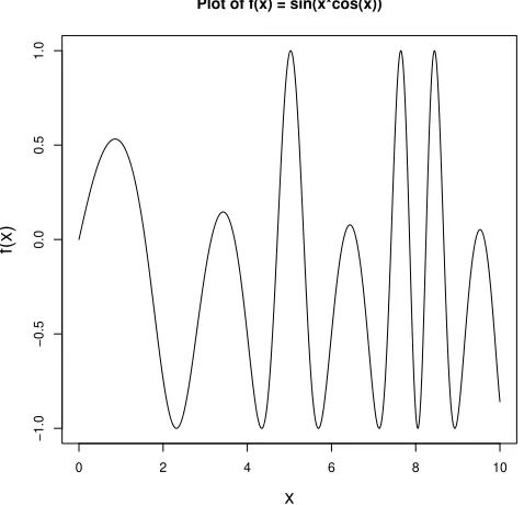
Plot of f(x) = sin(x*cos(x))
x
f(x)
Figure 1: sin(
x
cos(
x
)) for
x
∈
(0
,
10)
# we supply negative f, since we want to maximize.
f <- function(x) -exp(-( (x-2)^2 ))
######### without derivative
# I am using 1 at the initial value
# $par extracts only the argmax and nothing else
optim(1, f)$par
######### with derivative
df <- function(x) -2*(x-2)*f(x)
optim(1, f, df, method="CG")$par
Notice the derivative free method appears more sensitive to the starting value and gives
a warning message. But, the converged point looks about right when the starting value
is reasonable.
Example 2:
Suppose
f
(
x
) = sin(
x
cos(
x
)). This function has many local optimums.
Let’s see how
optim
finds minimums of this function which appear to occur around 2.1,
4.1, 5.8, and several others.
f <- function(x) sin(x*cos(x))
optim(2, f)$par
x
1.3 Two dimensional examples
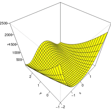
Example 3:
Let
f
(
x, y
) = (1
−
x
)
2+ 100(
y
−
x
2)
2, which is called the Rosenbrock
function. Let’s plot the function.
f <- function(x1,y1) (1-x1)^2 + 100*(y1 - x1^2)^2
x <- seq(-2,2,by=.15)
y <- seq(-1,3,by=.15)
z <- outer(x,y,f)
persp(x,y,z,phi=45,theta=-45,col="yellow",shade=.00000001,ticktype="detailed")
This function is strictly positive, but is 0 when
y
=
x
2, and
x
= 1, so (1
,
1) is a
min-imum. Let’s see if
optim
can figure this out. When using
optim
for multidimensional
optimization, the input in your function definition must be a single vector.
f <- function(x) (1-x[1])^2 + 100*(x[2]-x[1]^2)^2
# starting values must be a vector now
optim( c(0,0), f )$par
[1] 0.9999564 0.9999085
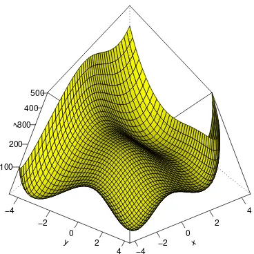
Example 4:
Let
f
(
x, y
) = (
x
2+
y
−
11)
2+ (
x
+
y
2−
7)
2, which is called Himmelblau’s
function. The function is plotted from belowin figure 3 by:
f <- function(x1,y1) (x1^2 + y1 - 11)^2 + (x1 + y1^2 - 7)^2
x <- seq(-4.5,4.5,by=.2)
x −4 −2
0 2
4
y −4
−2 0
2 4 z
100 200
300 400
500