Undergraduate Texts in Mathematics
Undergraduate Texts in Mathematics
(continued after index) Abbott:Understanding Analysis.
Anglin:Mathematics: A Concise History and Philosophy. Axler:Linear Algebra Done Right. Second
edition.
Beardon:Limits: A New Approach to Real Analysis.
Bak/Newman:Complex Analysis. Second edition.
Banchoff/Wermer:Linear Algebra Through Geometry. Second edition.
Berberian:A First Course in Real Analysis. Bix:Conics and Cubics: A Concrete
Introduction to Algebraic Curves.
Callahan:The Geometry of Spacetime: An Introduction to Special and General Relavitity.
Carter/van Brunt:The Lebesgue– Stieltjes Integral: A Practical Introduction. Cederberg:A Course in Modern Geometries.
Second edition.
Chambert-Loir:A Field Guide to Algebra Childs:A Concrete Introduction to Higher
Algebra. Second edition.
Chung/AitSahlia:Elementary Probability Theory: With Stochastic Processes and an Introduction to Mathematical Finance. Proving: A Closer Look at Mathematics. Devlin:The Joy of Sets: Fundamentals
of Contemporary Set Theory. Second edition. Dixmier:General Topology.
Erdõs/Surányi:Topics in the Theory of Numbers.
Estep:Practical Analysis on One Variable. Exner:An Accompaniment to Higher
Ghorpade/Limaye:A Course in Calculus and Real Analysis Hijab:Introduction to Calculus and Classical
Analysis.
Hilton/Holton/Pedersen:Mathematical Reflections: In a Room with Many Mirrors.
Sudhir R. Ghorpade
Balmohan V. Limaye
A Course in Calculus
and Real Analysis
Sudhir R. Ghorpade Department of Mathematics
Indian Institute of Technology Bombay Powai, Mumbai 400076
INDIA
Balmohan V. Limaye Department of Mathematics
Indian Institute of Technology Bombay Powai, Mumbai 400076
INDIA
Mathematics Subject Classification (2000): 26-01 40-XX
Library of Congress Control Number: 2006920312
ISBN-10: 0-387-30530-0 Printed on acid-free paper. ISBN-13: 978-0387-30530-1
© 2006 Springer Science+Business Media, LLC
All rights reserved. This work may not be translated or copied in whole or in part without the written permission of the publisher (Springer Science+Business Media, LLC, 233 Spring Street, New York, NY 10013, USA), except for brief excerpts in connection with reviews or scholarly analysis. Use in connection with any form of information storage and retrieval, electronic adap-tation, computer software, or by similar or dissimilar methodology now known or hereafter developed is forbidden.
The use in this publication of trade names, trademarks, service marks, and similar terms, even if they are not identified as such, is not to be taken as an expression of opinion as to whether or not they are subject to proprietary rights.
Printed in the United States of America. (MVY)
9 8 7 6 5 4 3 2 1
springer.com
Series Editors:
S. Axler
Mathematics Department San Francisco State University San Francisco, CA 94132 USA
K. A. Ribet
Department of Mathematics University of California at Berkeley Berkeley, CA 94720-3840
USA
Preface
Calculus is one of the triumphs of the human mind. It emerged from inves-tigations into such basic questions as finding areas, lengths and volumes. In the third century B.C., Archimedes determined the area under the arc of a parabola. In the early seventeenth century, Fermat and Descartes studied the problem of finding tangents to curves. But the subject really came to life in the hands of Newton and Leibniz in the late seventeenth century. In partic-ular, they showed that the geometric problems of finding the areas of planar regions and of finding the tangents to plane curves are intimately related to one another. In subsequent decades, the subject developed further through the work of several mathematicians, most notably Euler, Cauchy, Riemann, and Weierstrass.
Today, calculus occupies a central place in mathematics and is an essential component of undergraduate education. It has an immense number of appli-cations both within and outside mathematics. Judged by the sheer variety of the concepts and results it has generated, calculus can be rightly viewed as a fountainhead of ideas and disciplines in mathematics.
Real analysis, often called mathematical analysis or simply analysis, may be regarded as a formidable counterpart of calculus. It is a subject where one revisits notions encountered in calculus, but with greater rigor and sometimes with greater generality. Nonetheless, the basic objects of study remain the same, namely, real-valued functions of one or several real variables.
VI Preface
the circumference of a circle to its diameter is the same for all circles. It is our experience that a majority of students are unable to absorb these concepts and results without getting into vicious circles. This may partly be due to the division of calculus and real analysis in compartmentalized courses. Calculus is often taught as a service course and as such there is little time to dwell on subtleties and gain perspective. On the other hand, real analysis courses may start at once with metric spaces and devote more time to pathological exam-ples than to consolidating students’ knowledge of calculus. A host of topics such as L’Hˆopital’s rule, points of inflection, convergence criteria for Newton’s method, solids of revolution, and quadrature rules, which may have been in-adequately covered in calculus courses, become pass´e when one studies real analysis. Trigonometric, exponential, and logarithmic functions are defined, if at all, in terms of infinite series, thereby missing out on purely algebraic moti-vations for introducing these functions. The ubiquitous role ofπas a ratio of various geometric quantities and as a constant that can be defined indepen-dently using calculus is often not well understood. A possible remedy would be to avoid the separation of calculus and real analysis into seemingly disjoint courses and textbooks. Attempts along these lines have been made in the past as in the excellent books of Hardy and of Courant and John. Ours is another attempt to give a unified exposition of calculus and real analysis and address the concerns expressed above. While this book deals with functions of one variable, we intend to treat functions of several variables in another book.
The genesis of this book lies in the notes we prepared for an undergraduate course at the Indian Institute of Technology Bombay in 1997. Encouraged by the feedback from students and colleagues, the notes and problem sets were put together in March 1998 into a booklet that has been in private circulation. Initially, it seemed that it would be relatively easy to convert that booklet into a book. Seven years have passed since then and we now know a little better! While that booklet was certainly helpful, this book has evolved to acquire a form and philosophy of its own and is quite distinct from the original notes.
A glance at the table of contents should give the reader an idea of the topics covered. For the most part, these are standard topics and novelty, if any, lies in how we approach them. Throughout this text we have sought to make a distinction between the intrinsic definition of a geometric notion and the analytic characterizations or criteria that are normally employed in studying it. In many cases we have used articles such as those inA Century of Calculus to simplify the treatment. Usually each important result is followed by two kinds of examples: one to illustrate the result and the other to show that a hypothesis cannot be dropped.
Preface VII
within the text appear in square brackets. A list of symbols and abbreviations used in the text appears after the list of references.
TheNotes and Comments that appear at the end of each chapter are an important part of the book. Distinctive features of the exposition are men-tioned here and often pointers to some relevant literature and further devel-opments are provided. We hope that these may inspire many fruitful visits to the library—not when a quiz or the final is around the corner, but per-haps after it is over. TheNotes and Comments are followed by a fairly large collection of exercises. These are divided into two parts. Exercises in Part A are relatively routine and should be attempted by all students. Part B con-tains problems that are of a theoretical nature or are particularly challenging. These may be done at leisure. Besides the two sets of exercises in every chap-ter, there is a separate collection of problems, called Revision Exercises which appear at the end of Chapter 7. It is in Chapter 7 that the logarithmic, ex-ponential, and trigonometric functions are formally introduced. Their use is strictly avoided in the preceding chapters. This meant that standard examples and counterexamples such asxsin(1/x) could not be discussed earlier. The Revision Exercises provide an opportunity to revisit the material covered in Chapters 1–7 and to work out problems that involve the use of elementary transcendental functions.
The formal prerequisites for this course do not go beyond what is normally covered in high school. No knowledge of trigonometry is assumed and expo-sure to linear algebra is not taken for granted. However, we do expect some mathematical maturity and an ability to understand and appreciate proofs. This book can be used as a textbook for a serious undergraduate course in calculus. Parts of the book could be useful for advanced undergraduate and graduate courses in real analysis. Further, this book can also be used for self-study by students who wish to consolidate their knowledge of calculus and real analysis. For teachers and researchers this may be a useful reference for topics that are usually not covered in standard texts.
Apart from the first paragraph of this preface, we have not discussed the history of the subject or placed each result in historical context. However, we do not doubt that a knowledge of the historical development of concepts and results is important as well as interesting. Indeed, it can greatly enrich one’s understanding and appreciation of the subject. For those interested, we encourage looking on the Internet, where a wealth of information about the history of mathematics and mathematicians can be readily found. Among the various sources available, we particularly recommend the MacTutor History of Mathematics archive http://www-groups.dcs.st-and.ac.uk/history/ at the University of St. Andrews. The books of Boyer, Edwards, and Stillwell are also excellent sources for the history of mathematics, especially calculus.
VIII Preface
on this book. Financial assistance for the preparation of this book was re-ceived from the Curriculum Development Cell at IIT Bombay, for which we are thankful. Several colleagues and students have read parts of this book and have pointed out errors in earlier versions and made a number of useful suggestions. We are indebted to all of them and we mention, in particular, Rafikul Alam, Swanand Khare, Rekha P. Kulkarni, Narayanan Namboodri, S. H. Patil, Tony J. Puthenpurakal, P. Shunmugaraj, and Gopal K. Srinivasan. The figures in the book have been drawn usingPSTricks, and this is the work of Habeeb Basha and to a greater extent of Arunkumar Patil. We appreciate their efforts, and are grateful to them. Thanks are also due to C. L. Anthony, who typed a substantial part of the manuscript. The editorial and TeXnical staff at Springer, New York, have always been helpful and we thank all of them, especially Ina Lindemann and Mark Spencer for believing in us and for their patience and cooperation. We are also grateful to David Kramer, who did an excellent job of copyediting and provided sound counsel on linguistic and stylistic matters. We owe more than gratitude to Sharmila Ghorpade and Nirmala Limaye for their support.
We would appreciate receiving comments, suggestions, and corrections. These can be sent by e-mail to [email protected] or by writing to either of us. Corrections, modifications, and relevant information will be posted at http://www.math.iitb.ac.in/∼srg/acicara and we encourage interested readers to visit this website to learn about updates concerning the book.
Mumbai, India Sudhir Ghorpade
Contents
1 Numbers and Functions . . . 1
1.1 Properties of Real Numbers . . . 2
1.2 Inequalities . . . 10
1.3 Functions and Their Geometric Properties . . . 13
Exercises . . . 31
2 Sequences . . . 43
2.1 Convergence of Sequences . . . 43
2.2 Subsequences and Cauchy Sequences . . . 55
Exercises . . . 60
3 Continuity and Limits . . . 67
3.1 Continuity of Functions . . . 67
3.2 Basic Properties of Continuous Functions . . . 72
3.3 Limits of Functions of a Real Variable . . . 81
Exercises . . . 96
4 Differentiation. . . 103
4.1 The Derivative and Its Basic Properties . . . 104
4.2 The Mean Value and Taylor Theorems . . . 117
4.3 Monotonicity, Convexity, and Concavity . . . 125
4.4 L’Hˆopital’s Rule . . . 131
Exercises . . . 138
5 Applications of Differentiation. . . 147
5.1 Absolute Minimum and Maximum . . . 147
5.2 Local Extrema and Points of Inflection . . . 150
5.3 Linear and Quadratic Approximations . . . 157
5.4 The Picard and Newton Methods . . . 161
X Contents
6 Integration . . . 179
6.1 The Riemann Integral . . . 179
6.2 Integrable Functions . . . 189
6.3 The Fundamental Theorem of Calculus . . . 200
6.4 Riemann Sums . . . 211
Exercises . . . 218
7 Elementary Transcendental Functions . . . 227
7.1 Logarithmic and Exponential Functions . . . 228
7.2 Trigonometric Functions . . . 240
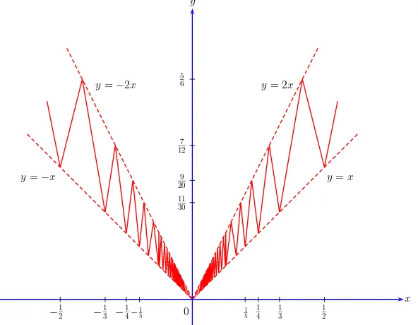
7.3 Sine of the Reciprocal . . . 253
7.4 Polar Coordinates . . . 260
7.5 Transcendence . . . 269
Exercises . . . 274
Revision Exercises . . . 284
8 Applications and Approximations of Riemann Integrals. . . . 291
8.1 Area of a Region Between Curves . . . 291
8.2 Volume of a Solid . . . 298
8.3 Arc Length of a Curve . . . 311
8.4 Area of a Surface of Revolution . . . 318
8.5 Centroids . . . 324
8.6 Quadrature Rules . . . 336
Exercises . . . 352
9 Infinite Series and Improper Integrals . . . 361
9.1 Convergence of Series . . . 361
9.2 Convergence Tests for Series . . . 367
9.3 Power Series . . . 376
9.4 Convergence of Improper Integrals . . . 384
9.5 Convergence Tests for Improper Integrals . . . 392
9.6 Related Integrals . . . 398
Exercises . . . 410
References. . . 419
List of Symbols and Abbreviations. . . 423
1
Numbers and Functions
Let us begin at the beginning. When we learn the script of a language, such as the English language, we begin with the letters of the alphabet A, B, C, . . .; when we learn the sounds of music, such as those of western classical music, we begin with the notes Do, Re, Mi, . . . . Likewise, in mathematics, one begins with 1,2,3, . . .; these are the positive integers or the natural numbers. We shall denote the set of positive integers by N. Thus,
N={1,2,3, . . .}.
These numbers have been known since antiquity. Over the years, the number 0 was conceived1and subsequently, the negative integers. Together, these form
the setZof integers.2Thus,
Z={. . . ,−3,−2,−1,0,1,2,3, . . .}.
Quotients of integers are calledrational numbers. We shall denote the set of all rational numbers byQ. Thus,
Q=m
n :m, n∈Z, n= 0
.
Geometrically, the integers can be represented by points on a line by fixing a base point (signifying the number 0) and a unit distance. Such a line is called thenumber lineand it may be drawn as in Figure 1.1. By suitably subdi-viding the segment between 0 and 1, we can also represent rational numbers such as 1/n, wheren ∈ N, and this can, in turn, be used to represent any
1
The invention of ‘zero’, which also paves the way for the place value system of enumeration, is widely credited to the Indians. Great psychological barriers had to be overcome when ‘zero’ was being given the status of a legitimate number. For more on this, see the books of Kaplan [39] and Kline [41].
2
2 1 Numbers and Functions
Fig. 1.1.The number line
rational number by a unique point on the number line. It is seen that the rational numbers spread themselves rather densely on this line. Nevertheless, several gaps do remain. For example, the ‘number’√2 can be represented by a unique point between 1 and 2 on the number line using simple geometric constructions, but as we shall see later, this is not a rational number. We are, therefore, forced to reckon with the so-called irrational numbers, which are precisely the ‘numbers’ needed to fill the gaps left on the number line after marking all the rational numbers. The rational numbers and the irrational numbers together constitute the set R, called the set of real numbers. The geometric representation of the real numbers as points on the number line naturally implies that there is anorder among the real numbers. In particu-lar, those real numbers that are greater than 0, that is, which correspond to points to the right of 0, are calledpositive.
1.1 Properties of Real Numbers
To be sure, we haven’t precisely defined what real numbers are and what it means for them to be positive. For that matter, we haven’t even defined the positive integers 1,2,3, . . .or the rational numbers.3 But at least we are familiar with the latter. We are also familiar with the addition and the mul-tiplication of rational numbers. As for the real numbers, which are not easy to define, it is better to at least specify the properties that we shall take for granted. We shall take adequate care that in the subsequent development, we use only these properties or the consequences derived from them. In this way, we don’t end up taking too many things on faith. So let us specify our assumptions.
We assume that there is a set R (whose elements are called real num-bers), which contains the set Q of all rational numbers (and, in particular, the numbers 0 and 1) such that the following three types of properties are satisfied.
3
1.1 Properties of Real Numbers 3
Algebraic Properties
We have the operations of addition (denoted by +) and multiplication (de-noted by · or by juxtaposition) on R, which extend the usual addition and multiplication of rational numbers and satisfy the following properties: A1 a+ (b+c) = (a+b) +cand a(bc) = (ab)c for alla, b, c∈R.
A2 a+b=b+a andab=ba for alla, b∈R.
A3 a+ 0 =aanda·1 =afor all a∈R.
A4 Given any a∈R, there is a′ ∈Rsuch that a+a′= 0. Further, if a= 0,
then there is a∗∈Rsuch thataa∗= 1.
A5 a(b+c) =ab+ac for alla, b, c∈R.
It is interesting to note that several simple properties of real numbers that one is tempted to take for granted can be derived as consequences of the above properties. For example, let us prove thata·0 = 0 for alla∈R. First, by A3, we have 0 + 0 = 0. So, by A5,a·0 =a(0 + 0) =a·0 +a·0. Now, by A4, there is ab′∈Rsuch thata·0 +b′= 0. Thus,
0 =a·0 +b′= (a·0 +a·0) +b′=a·0 + (a·0 +b′) =a·0 + 0 =a·0,
where the third equality follows from A1 and the last equality follows from A3. This completes the proof! A number of similar properties are listed in the exercises and we invite the reader to supply the proofs. These show, in particular, that given anya∈R, an elementa′ ∈Rsuch that a+a′ = 0 is
unique; this element will be called thenegativeor the additive inverseof aand denoted by−a. Likewise, if a∈Randa= 0, then an elementa∗ ∈R
such that aa∗ = 1 is unique; this element is called the reciprocal or the
multiplicative inverseofaand is denoted bya−1or by 1/a. Once all these
formalities are understood, we will be free to replace expressions such as
a(1/b), a+a, aa, (a+b) +c, (ab)c, a+ (−b),
by the corresponding simpler expressions, namely,
a/b, 2a, a2, a+b+c, abc, a
−b.
Here, for instance, it is meaningful and unambiguous to writea+b+c, thanks to A1. More generally, given finitely many real numbers a1, . . . , an, the sum
a1+· · ·+an has an unambiguous meaning. To represent such sums, the
“sigma notation” can be quite useful. Thus,a1+· · ·+an is often denoted by
n
i=1aior sometimes simply byiaiorai. Likewise, the producta1· · ·an
of the real numbers a1, . . . , an has an unambiguous meaning and it is often
denoted byni=1ai or sometimes simply byiai orai. We remark that as
4 1 Numbers and Functions
Order Properties
The set Rcontains a subset R+, called the set of all positive real numbers,
satisfying the following properties:
O1 Given any a∈R, exactly one of the following statements is true:
a∈R+; a= 0; −a∈R+. O2 If a, b∈R+, thena+b
∈R+ and ab
∈R+.
Given the existence ofR+, we can define anorder relationonRas follows.
For a, b ∈ R, define a to be less than b, and write a < b, if b−a ∈ R+.
Sometimes, we writeb > ain place ofa < band say thatb isgreater than a. With this notation, it follows from the algebraic properties that R+ =
{x∈R:x >0}. Moreover, the following properties are easy consequences of A1–A5 and O1–O2:
(i) Given anya, b∈R, exactly one of the following statements is true.
a < b; a=b; b < a.
(ii) Ifa, b, c∈Rwitha < b andb < c, then a < c.
(iii) Ifa, b, c∈R, witha < b, thena+c < b+c. Further, ifc >0, thenac < bc, whereas if c <0, thenac > bc.
Note that it is also a consequence of the properties above that 1>0. Indeed, by (i), we have either 1>0 or 1 < 0. If we had 1<0, then we must have
−1 > 0 and hence by (iii), 1 = (−1)(−1) > 0, which is a contradiction. Therefore, 1>0. A similar argument shows thata2>0 for anya
∈R,a= 0. The notation a ≤ b is often used to mean that either a < b or a = b. Likewise,a≥bmeans that a > bora=b.
LetS be a subset ofR. We say that S isbounded above if there exists α∈Rsuch that x≤αfor allx∈S. Any suchαis called anupper bound ofS. We say thatSisbounded belowif there existsβ ∈Rsuch thatx≥β for allx∈S. Any suchβ is called alower boundof S. The setS is said to be boundedif it is bounded above as well as bounded below; otherwise, S is said to be unbounded. Note that if S =∅, that is, if S is the empty set, then every real number is an upper bound as well as a lower bound ofS.
Examples 1.1. (i) The setNof positive integers is bounded below, and any real number β ≤1 is a lower bound of N. However, as we shall see later in Proposition 1.3, the setNis not bounded above.
(ii) The setS of reciprocals of positive integers, that is,
S:=
1,1 2,
1 3, . . .
1.1 Properties of Real Numbers 5
(iii) The set S := {x ∈ Q: x2 < 2} is bounded. Here, for example, 2 is an
upper bound, while−2 is a lower bound. ✸ Let S be a subset ofR. An element M ∈ Ris called a supremumor a least upper boundof the setS if
(i) M is an upper bound ofS, that is,x≤M for allx∈S, and (ii) M ≤αfor any upper boundαof S.
It is easy to see from the definition that ifShas a supremum, then it must be unique; we denote it by supS. Note that∅ does not have a supremum.
An elementm∈Ris called aninfimumor agreatest lower boundof the setS if
(i) mis a lower bound ofS, that is,m≤xfor allx∈S, and (ii) β ≤m for any lower boundβ ofS.
Again, it is easy to see from the definition that ifShas an infimum, then it must be unique; we denote it by infS. Note that∅does not have an infimum. For example, ifS={x∈R: 0< x≤1}, then infS= 0 and supS= 1. In this example, infS is not an element ofS, but supS is an element ofS.
If the supremum of a setS is an element ofS, then it is called the maxi-mumofS, and denoted by maxS; likewise, if the infimum ofS is inS, then it is called theminimumofS, and denoted by minS.
The last, and perhaps the most important, property of R that we shall assume is the following.
Completeness Property
Every nonempty subset ofRthat is bounded above has a supremum.
The significance of the Completeness Property (which is also known as the Least Upper Bound Property) will become clearer from the results proved in this as well as the subsequent chapters.
Proposition 1.2.Let S be a nonempty subset of R that is bounded below. Then S has an infimum.
Proof. LetT ={β ∈ R: β ≤a for alla∈S}. SinceS is bounded below,T is nonempty, and since S is nonempty, T is bounded above. Hence T has a supremum. It is easily seen that supT is the infimum ofS. ⊓⊔
Proposition 1.3.Given any x∈ R, there is somen ∈ N such that n > x. Consequently, there is also anm∈N such that−m < x.
Proof. Assume the contrary. Thenxis an upper bound ofN. Therefore,Nhas a supremum. LetM = supN. ThenM −1 < M and henceM −1 is not an upper bound ofN. So, there isn∈Nsuch thatM−1< n. But thenn+ 1∈N
6 1 Numbers and Functions
The first assertion in the proposition above is sometimes referred to as the Archimedean propertyofR. Observe that for any positive real numberǫ, by applying the Proposition 1.3 to x= 1/ǫ, we see that there exists n ∈N
such that (1/n)< ǫ. Note also that thanks to Proposition 1.3, for anyx∈R, there are m, n ∈ Nsuch that −m < x < n. The largest among the finitely many integersk satisfying−m≤k≤n and alsok≤xis called the integer partofxand is denoted by [x]. Note that the integer part ofxis characterized by the following properties:
[x]∈Z and [x]≤x <[x] + 1.
Sometimes, the integer part of xis called the floor of xand is denoted by
⌊x⌋. In the same vein, the smallest integer≥xis called theceilingofxand is denoted by⌈x⌉. For example,⌊3
2⌋=⌊1⌋= 1, whereas
3 2
=⌈2⌉= 2.
Given any a ∈ R and n ∈ N, we define the nth power an of a to be
the producta· · ·aof a with itself takenn times. Further, we definea0 = 1
anda−n= (1/a)n provideda= 0. In this way integral powers of all nonzero
real numbers are defined. The following elementary properties are immediate consequences of the algebraic properties and the order properties ofR.
(i) (a1a2)n=an1an2 for alln∈Zanda1, a2∈R(witha1a2= 0 ifn≤0).
(ii) (am)n
=amn and am+n=aman for allm, n
∈Zand a∈R(with a= 0 ifm≤0 orn≤0).
(iii) Ifn∈Nandb1, b2∈Rwith 0≤b1< b2, thenbn1 < bn2.
The first two properties above are sometimes called thelaws of exponents or thelaws of indices(for integral powers).
Proposition 1.4.Given any n ∈ N and a ∈ R with a ≥ 0, there exists a uniqueb∈Rsuch thatb≥0andbn=a.
Proof. Uniqueness is clear since b1, b2 ∈ R with 0 ≤ b1 < b2 implies that
bn
1 < bn2. To prove the existence ofb∈Rwithb≥0 andbn=a, note that the
case ofa= 0 is trivial, and moreover, the case of 0< a <1 follows from the case ofa >1 by taking reciprocals. Thus we will assume thata≥1. Let
Sa={x∈R:xn ≤a}.
Then Sa is a subset of R, which is nonempty (since 1 ∈ Sa) and bounded
above (bya, for example). Defineb= supSa. Note that since 1∈Sa, we have
b≥1>0. We will show thatbn=aby showing that each of the inequalities
bn < aandbn> aleads to a contradiction.
Note that by Binomial Theorem, for any δ∈R, we have
(b+δ)n=bn+ n 1
bn−1δ+ n 2
1.1 Properties of Real Numbers 7
Now, supposebn< a. Let us define
ǫ:=a−bn, M := max n k
bn−k:k= 1, . . . , n
and δ:= min1, ǫ nM
.
ThenM ≥1 and 0< δk
≤δ fork= 1,2, . . . , n. Therefore,
(b+δ)n≤bn+M δ+M δ2+· · ·+M δn≤bn+nM δ≤bn+ǫ=a. Hence,b+δ∈Sa. But this is a contradiction sincebis an upper bound ofSa.
Next, suppose bn > a. This time, takeǫ=bn
−aand defineM andδ as before. Similar arguments will show that
(b−δ)n≥bn−nM δ≥bn−ǫ=a.
Butb−δ < b, and henceb−δcannot be an upper bound ofSa. This means
that there is somex∈Sa such that b−δ < x. Therefore, (b−δ)n < xn ≤a,
which is a contradiction. Thusbn=a. ⊓⊔
Thanks to Proposition 1.4, we define, for anyn∈Nanda∈Rwitha≥0, thenthrootofato be the unique real numberbsuch thatb≥0 andbn=a;
we denote this real number by √na or by a1/n. In case n = 2, we simply write√ainstead of √2a. From the uniqueness of the nth root, the analogues of the properties (i), (ii), and (iii) stated just before Proposition 1.4 can be easily proved fornth roots instead of thenth powers. More generally, given any r∈Q, we writer=m/n, wherem, n∈Zwithn >0, and definear= (am)1/n for anya∈R witha >0. Note that if also r =p/q, for somep, q∈Z with q > 0, then for any a ∈ R with a > 0, we have (am)1/n
= (ap)1/q
. This can be seen, for example, by raising both sides to thenqth power, using laws of exponents for integral powers and the uniqueness of roots. Thus, rational powers of positive real numbers are unambiguously defined. In general, for negative real numbers, nonintegral rational powers are not defined inR. For example, (−1)1/2cannot equal any b∈Rsinceb2 ≥0. However, in a special
case, rational powers of negative real numbers can be defined. More precisely, ifn∈Nis odd anda∈Ris positive, then we define
(−a)1/n=
−a1/n.
It is easily seen that this is well defined, and as a result, for any x ∈ R, x= 0, therthpowerxris defined wheneverr
∈Qhas an odd denominator, that is, when r = m/n for some m ∈ Z and n ∈ N with n odd. Finally, if r is any positive rational number, then we set 0r = 0. For rational powers,
8 1 Numbers and Functions
Real numbers that are not rational numbers are calledirrational num-bers. The possibility of taking nth roots provides a useful method to con-struct several examples of irrational numbers. For instance, we prove below a classical result that√2 is an irrational number. The proof here is such that it can easily be adapted to prove that several such numbers, for example,
√
3,√15,√3 2,√5
16, are not rational. [See Exercises 10 and 44.] We recall first the familiar notion of divisibility in the set Z of integers. Given m, n ∈ Z, we say that m divides n or that m is a factor of n (and write m | n) if n=ℓm for some ℓ ∈Z. Sometimes, we write m ∤n ifm does not divide n. Two integersm and n are said to berelatively prime if the only integers that divide bothm andnare 1 and−1. It can be shown that ifm, n, n′ ∈Z
are such thatm, nare relatively prime and m|nn′, thenm|n′. It can also
be shown that any rational numberrcan be written as
r= p
q, wherep, q∈Z, q >0, andp, q are relatively prime.
The above representation ofris called thereduced formofr. The numerator (namely,p) and the denominator (namely, q) in the case of a reduced form representation are uniquely determined byr.
Proposition 1.5.No rational number has a square equal to2. In other words,
√
2 is an irrational number.
Proof. Suppose√2 is rational. Write√2 in the reduced form asp/q, where p, q∈Z,q >0, andp, q are relatively prime. Thenp2= 2q2. Henceq divides
p2. This implies that q divides p, and so p/q is an integer. But there is no
integer whose square is 2 because (±1)2 = 1 and the square of any integer
other than 1 or−1 is ≥4. Hence√2 is not rational. ⊓⊔
The following result shows that the rational numbers as well as the irra-tional numbers spread themselves rather densely on the number line.
Proposition 1.6.Given any a, b ∈ R with a < b, there exists a rational number as well as an irrational number between aandb.
Proof. By Proposition 1.3, we can findn ∈ Nsuch that n > 1/(b−a). Let m= [na] + 1. Thenm−1≤na < m, and hence
a < m
n ≤
na+ 1
n =a+
1
n < a+ (b−a) =b.
Thus we have found a rational number (namely,m/n) betweenaandb. Now, a+√2< b+√2, and ifris a rational number betweena+√2 andb+√2, thenr−√2 is an irrational number betweenaandb. ⊓⊔
1.1 Properties of Real Numbers 9
(a, b) :={x∈R:a < x < b}
and theclosed intervalfrom atobto be the set
[a, b] :={x∈R:a≤x≤b}.
Thesemiopenor thesemiclosedintervals from atobare defined by
(a, b] :={x∈R:a < x≤b} and [a, b) :={x∈R:a≤x < b}.
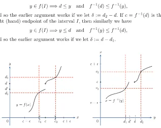
In other words, (a, b] := [a, b]\ {a}and [a, b) := [a, b]\ {b}. Note that ifa > b, then each of these intervals is empty, whereas ifa=b, then [a, b] ={a}while the other intervals froma to b are empty. If I is a subset of R of the form [a, b], (a, b), [a, b) or (a, b], wherea, b∈Rwitha < b, thenais called theleft (hand) endpointof I while b is called the right (hand) endpointof I. Collectively,aandbare called theendpointsofI.
It is often useful to consider the symbols ∞ (called infinity) and −∞
(called minus infinity), which may be thought as the fictional (right and left) endpoints of the number line. Thus
−∞< a <∞ for alla∈R.
The set R together with the additional symbols ∞ and −∞ is sometimes called the set ofextended real numbers. We use the symbols∞and−∞ to define, for anya∈R, the followingsemi-infinite intervals:
(−∞, a) :={x∈R:x < a}, (−∞, a] :={x∈R:x≤a}
and
(a,∞) :={x∈R:x > a}, [a,∞) :={x∈R:x≥a}.
The set R can also be thought of as the doubly infinite interval (−∞,∞), and as such we may sometimes use this interval notation for the set of all real numbers.
It may be noted that each of the above types of intervals has a basic property in common. We state this in the form of the following definition.
LetI⊆R, that is, letI be a subset ofR. We say thatI is anintervalif
a, b∈I anda < b=⇒[a, b]⊆I.
In other words, the line segment connecting any two points ofI is inI. This is sometimes expressed by saying that an interval is a ‘connected set’.
10 1 Numbers and Functions
Proof. IfI=∅, thenI= (a, a) for anya∈R. SupposeI=∅. Define
a:=
infI ifI is bounded below,
−∞ otherwise, andb:=
supI ifIis bounded above,
∞ otherwise.
Note that by the Completeness Property and Proposition 1.2, botha and b are well defined anda≤b. SinceI is an interval, it follows that
(i)I= (a, b), or (ii)I= [a, b], or (iii) I= [a, b), or (iv)I= (a, b],
according as (i)a∈Iandb∈I, or (ii)a∈Iandb∈I, or (iii)a∈Iandb∈I, or (iv)a∈I andb∈I. This proves the proposition. ⊓⊔
In the proof of the above proposition, we have considered intervals that can reduce to the empty set or to a set containing only one point. However, to avoid trivialities, we shall usually refrain from doing so in the sequel. Henceforth, when we write [a, b], (a, b), [a, b) or (a, b], it will be tacitly assumed thataand bare real numbers anda < b.
Given any real number a, the absolute value or themodulus of a is denoted by|a|and is defined by
|a|:=
a if a≥0,
−a if a <0.
Note that|a| ≥0,|a|=| −a|, and|ab|=|a| |b| for anya, b∈R. The notion of absolute value can sometimes be useful in describing certain intervals that are symmetric about a point. For example, if a∈R and ǫ is a positive real number, then
(a−ǫ, a+ǫ) ={x∈R:|x−a|< ǫ}.
1.2 Inequalities
In this section, we describe and prove some inequalities that will be useful to us in the sequel.
Proposition 1.8 (Basic Inequalities for Absolute Values). Given any
a, b∈R, we have
(i)|a+b| ≤ |a|+|b|,
(ii)| |a| − |b| | ≤ |a−b|.
Proof. It is clear that a≤ |a| and b ≤ |b|. Thus, a+b ≤ |a|+|b|. Likewise,
−(a+b)≤ |a|+|b|. This implies (i). To prove (ii), note that by (i), we have
1.2 Inequalities 11
The first inequality in the proposition above is sometimes referred to as the triangle inequality. An immediate consequence of this is that ifa1, . . . , an
are any real numbers, then
|a1+a2+· · ·+an| ≤ |a1|+|a2|+· · ·+|an|.
Proposition 1.9 (Basic Inequalities for Powers and Roots). Given any a, b∈Randn∈N, we have
(i)|an
−bn
| ≤nMn−1
|a−b|, whereM = max{|a|,|b|},
(ii)|a1/n−b1/n| ≤ |a−b|1/n, provided a≥0 andb≥0. Proof. (i) Consider the identity
an−bn= (a−b)(an−1b+an−2b2+· · ·+a2bn−2+abn−1).
Take the absolute value of both sides and use Proposition 1.8. The absolute value of the second factor on the right is bounded above by nMn−1. This
implies the inequality in (i).
(ii) We may assume, without loss of generality, that a≥b. Letc =a1/n
andd=b1/n. Thenc
−d≥0 and by the Binomial Theorem, cn= [(c−d) +d]n= (c−d)n+· · ·+dn≥(c−d)n+dn. Therefore,
a−b=cn−dn≥(c−d)n= [a1/n−b1/n]n.
This implies the inequality in (ii). ⊓⊔
We remark that the basic inequality for powers in part (i) of Proposition 1.9 is valid, more generally, for rational powers. [See Exercise 54 (i).] As for part (ii), a slightly weaker inequality holds if instead ofnth roots, we consider rational roots. [See Exercise 54 (ii).]
Proposition 1.10 (Binomial Inequalities). Given any a ∈ R such that
1 +a≥0, we have
(1 +a)n ≥1 +na for all n∈N.
More generally, given any n∈N anda1, . . . , an∈R such that1 +ai ≥0 for
i= 1, . . . , n anda1, . . . , an all have the same sign, we have
(1 +a1)(1 +a2)· · ·(1 +an)≥1 + (a1+· · ·+an).
Proof. Clearly, the first inequality follows from the second by substituting a1 = · · · = an =a. To prove the second inequality, we use induction on n.
The case ofn= 1 is obvious. If n >1 and the result holds forn−1, then (1 +a1)(1 +a2)· · ·(1 +an)≥(1 +bn)(1 +an),
wherebn=a1+· · ·+an−1. Now,bn andan have the same sign, and hence
(1 +bn)(1 +an) = 1 +bn+an+bnan≥1 +bn+an.
12 1 Numbers and Functions
Note that the first inequality in the proposition above is an immediate consequence of the Binomial Theorem whena≥0, although we have proved it in the more general case of a ≥ −1. We shall refer to the first inequality in Proposition 1.10 as the binomial inequality. On the other hand, we shall refer to the second inequality in Proposition 1.10 as the generalized binomial inequality. We remark that the binomial inequality is valid, more generally, for rational powers. [See Exercise 54 (iii).]
Proposition 1.11 (A.M.-G.M. Inequality). Letn∈Nand leta1, . . . , an
be nonnegative real numbers. Then the arithmetic mean ofa1, . . . , anis greater
than or equal to their geometric mean, that is,
a1+· · ·+an
n ≥
n √a
1· · ·an.
Moreover, equality holds if and only if a1=· · ·=an.
Proof. If some ai = 0, then the result is obvious. Hence we shall assume
that ai > 0 for i = 1, . . . , n. Let g = (a1· · ·an)1/n and bi = ai/g for i =
1, . . . , n. Then b1, . . . , bn are positive andb1· · ·bn = 1. We shall now show,
using induction on n, that b1+· · ·+bn ≥ n. This is clear if n = 1 or if
each ofb1, . . . , bn equals 1. Suppose n > 1 and not every bi equals 1. Then
b1· · ·bn = 1 implies that among b1, . . . , bn there is a number <1 as well as
a number>1. Relabelingb1, . . . , bn if necessary, we may assume thatb1<1
andbn>1. Letc1=b1bn. Thenc1b2· · ·bn−1= 1, and hence by the induction
hypothesisc1+b2+· · ·+bn−1≥n−1. Now observe that
b1+· · ·+bn= (c1+b2+· · ·+bn−1) +b1+bn−c1
≥(n−1) +b1+bn−b1bn
=n+ (1−b1)(bn−1)
> n,
where the last inequality follows since b1 <1 and bn >1. This proves that
b1+· · ·+bn≥n, and moreover the inequality is strict unlessb1=· · ·=bn = 1.
Substituting bi=ai/g, we obtain the desired result. ⊓⊔
Proposition 1.12 (Cauchy–Schwarz Inequality). Let n ∈ N and let
a1, . . . , an andb1, . . . , bn be any real numbers. Then n
i=1
aibi≤
n
i=1
a2i
1/2n
i=1
b2i
1/2
.
Moreover, equality holds if and only if a1, . . . , an and b1, . . . , bn are
propor-tional to each other, that is, ifaibj =ajbi for all i, j= 1, . . . , n.
1.3 Functions and Their Geometric Properties 13
the terms in the second summation above, then we obtain
n
This proves the desired result. ⊓⊔
Remark 1.13.Analyzing the argument in the above proof of the Cauchy– Schwarz inequality, we obtain, in fact, the following identity, which is easy to verify directly:
This is known as Lagrange’s Identity and it may be viewed as a one-line proof of Proposition 1.12. See also Exercise 16 for yet another proof. ✸
1.3 Functions and Their Geometric Properties
The concept of a function is of basic importance in calculus and real analysis. In this section, we begin with an informal description of this concept followed by a precise definition. Next, we outline some basic terminology associated with functions. Later, we give basic examples of functions, including polyno-mial functions, rational functions, and algebraic functions. Finally, we discuss a number of geometric properties of functions and state some results concern-ing them. These results are proved here without invokconcern-ing any of the notions of calculus that are encountered in the subsequent chapters.
Typically, a function is described with the help of an expression in a single parameter (say x), which varies over a stipulated set; this set is called the
domainof that function. For example, each of the expressions
(i)f(x) := 2x+ 1, x∈R, (ii)f(x) :=x2, x∈R,
(iii)f(x) := 1/x, x∈R, x= 0, (iv)f(x) :=x3, x∈R,
14 1 Numbers and Functions
set R; to indicate this, we say that R is the codomain of these functions or that these arereal-valued functions.
Given a real-valued function f having a subset D of R as its domain, it is often useful to consider the graph of f, which is defined as the subset
{(x, f(x)) :x∈D}of the planeR2. In other words, this is the set of points on
thecurvegiven byy=f(x), x∈D, in thexy-plane. For example, the graphs of the functions in (i) and (ii) are shown in Figure 1.2, while the graphs of the functions in (iii) and (iv) above are shown in Figure 1.3.
2
1 3
0
−2 −1
−3
2 1 3 4
−2
−1
−3
−4
x y
y= 2x+ 1
2
1 3
0
−2 −1
−3
2 1 3 4
−2
−1
−3
−4
x y
y=x2
Fig. 1.2. Graphs off(x) = 2x+ 1 andf(x) =x2
In general, we can talk about a function from any setDto any setE, and this associates to each point ofDa unique element ofE. A formal definition of a function is given below. It may be seen that this, in essence, identifies a function with its graph!
Definitions and Terminology
LetD and E be any sets. We denote byD×E the set of all ordered pairs (x, y) wherexvaries over elements of D and y varies over elements ofE. A functionfromD toE is a subsetf ofD×E with the property that for each x∈D, there is a uniquey ∈E such that (x, y)∈f. The setD is called the domainor thesourceof f and Ethecodomainor thetargetoff.
Usually, we write f : D →E to indicate thatf is a function fromD to E. Also, instead of (x, y) ∈f, we usually write y =f(x), and call f(x) the valueoff atx. This may also be indicated by writingx→f(x), and saying that f mapsxtof(x). Functionsf :D→E andg :D→E are said to be equaland we write f =giff(x) =g(x) for allx∈D.
1.3 Functions and Their Geometric Properties 15
On the other hand, iff maps distinct points to distinct points, that is, if
x1, x2∈D, f(x1) =f(x2) =⇒x1=x2
thenf is said to beone-oneorinjective. Iff is both one-one and onto, then it is said to bebijectiveor aone-to-one correspondence.
The notion of a bijective function can be used to define a basic terminology concerning sets as follows. Given any nonnegative integern, consider the set
{1, . . . , n} of the firstnpositive integers. Note that ifn= 0, then{1, . . . , n} is the empty set. A setDis said to befiniteif there is a bijective map from
{1, . . . , n}ontoD, for some nonnegative integern. In this case the nonnegative integernis unique (Exercise 18) and it is called thecardinalityofD or the number of elementsinD. A set that is not finite is said to beinfinite.
1 2 3 4
−1
−2
−3
−4
2
1 3 4
−1
−2
−3
−4
x y
y= 1/x
2
1 3
0
−1
−2
−3
1 2 3 4
−1
−2
−3
−4
x y
y=x3
Fig. 1.3.Graphs off(x) = 1/x andf(x) =x3
The simplest examples of functions defined on arbitrary sets are an identity function and a constant function. Given any set D, the identity function on D is the function idD : D → D defined by idD(x) = x for all x ∈ D.
Given any sets D and E, a functionf :D → E defined by f(x) =c for all x∈D, wherec is a fixed element ofE, is called aconstant function. Note that idD is always bijective, whereas a constant function is neither one-one
(unlessD is a singleton set!) nor onto (unless E is a singleton set!). To look at more specific examples, note thatf :R→Rdefined by (i) or by (iv) above is bijective, whilef :R→[0,∞) defined by (ii) is onto but not one-one, and f :R\ {0} →Rdefined by (iii) is one-one but not onto.
If f : D → E and g : D′ → E′ are functions with f(D) ⊆ D′, then
the function h : D → E′ defined by h(x) = g(f(x)), x ∈ D, is called the
compositeofg withf, and is denoted byg◦f [read asgcomposed with f, or asf followed by g].
16 1 Numbers and Functions
done by looking at the function ˜f :D→f(D) defined by ˜f(x) =f(x), x∈D. In particular, iff :D →E is one-one, then for every y∈f(D), there exists a unique x ∈ D such that f(x) = y. In this case, we write x = f−1(y). We thus obtain a function f−1 : f(D)
→ D such that f−1
◦f = idD and
f◦f−1= id
f(D). We callf−1 theinverse function off.
For example, the inverse off :R→Rdefined by (i) above is the function f−1 :R
→Rgiven by f−1(y) = (y
−1)/2 fory ∈R, whereas the inverse of f :R\ {0} →Rdefined by (iii) above is the functionf−1:R
\ {0} →R\ {0} given byf−1(y) = 1/yfory
∈R\ {0}.
In general, if a function f : D →E is not one-one, then we cannot talk about its inverse. However, sometimes it is possible to restrict the domain of a function to a smaller set and then a ‘restriction’ off may become injective. For any subsetCofD, therestrictionoff toCis the functionf|C:C→E,
defined byf|C(x) =f(x) forx∈C. For example, iff :R→Ris the function
defined by (ii), thenf is not one-one but its restrictionf|[0,∞)is one-one and
its inverseg=f|[0,∞)− 1
is given byg(y) =√y fory∈[0,∞).
SupposeD⊆Rissymmetricabout the origin, that is, we have−x∈D wheneverx∈D. For example,D can be the whole real line Ror an interval of the form [−a, a] or the punctured real lineR\ {0}. A functionf :D →R
is said to be aneven functionif f(−x) =f(x) for allx∈D, whereas f is said to be anodd function if f(−x) =−f(x) for all x∈D. For example, f :R→Rdefined byf(x) =x2 is an even function, whereasf :R
\ {0} →R
defined by f(x) = 1/x and f : R → Rdefined by f(x) = x3 are both odd
functions. On the other hand,f :R→Rdefined by f(x) = 2x+ 1 is neither even nor odd.
Geometrically speaking, givenD⊆Rand f :D→R, the fact thatf is a function corresponds to the property that for everyx0∈D, the vertical line
x=x0in thexy-plane meets the graph off in exactly one point. Further, the
property thatf is one-one corresponds to requiring, in addition, that for any y0∈R, the horizontal liney =y0 meet the graph off in at most one point.
On the other hand, the property that a pointy0∈Ris in the rangef(D) off
corresponds to requiring, in addition, that the horizontal liney=y0meet the
graph off in at least one point. In case the inverse functionf−1:f(D)
→R
exists, then its graph is obtained from that offby reflecting along the diagonal liney =x. Assuming thatD is symmetric, to say that f is an even function corresponds to saying that the graph off is symmetric with respect to the y-axis, whereas to say thatf is an odd function corresponds to saying that the graph off is symmetric with respect to the origin. Notice that iff is odd and one-one, then its rangef(D) is also symmetric, andf−1 :f(D)→Ris
an odd function.
Given any real-valued functions f, g : D → R, we can associate new functions f +g :D → Rand f g :D →R, called respectively the sumand theproductoff andg, which are defined componentwise, that is, by
1.3 Functions and Their Geometric Properties 17
In casef is the constant function given by f(x) =cfor allx∈D, thenf g is often denoted bycgand called themultipleofg(byc). We often writef−g in place off + (−1)g. In case g(x) = 0 for all x ∈D, the quotient f /g is defined and this is a function fromDtoRgiven by (f /g) (x) =f(x)/g(x) for x∈D. Sometimes, we write f ≤g to mean that f(x)≤g(x) for allx∈D.
Basic Examples of Functions
Among the most basic functions are those that are obtained from polynomials. Let us first review some relevant algebraic facts about polynomials.
A polynomial(in one variablex) with real coefficients is an expression4
of the form
cnxn+cn−1xn−1+· · ·+c1x+c0,
wheren is a nonnegative integer andc0, c1, . . . , cn are real numbers. We call
c0, c1, . . . , cn thecoefficientsof the above polynomial and more specifically,
ci as thecoefficient ofxi fori= 0,1, . . . , n. In casecn = 0, the polynomial
is said to have degree n, and cn is said to be its leading coefficient. A
polynomial (in x) whose leading coefficient is 1 is said to bemonic (in x). Two polynomials are said to be equal if the corresponding coefficients are equal. In particular, cnxn +· · ·+c1x+c0 is the zero polynomial if and
only if c0 = c1 = · · · = cn = 0. The degree of the zero polynomial is not
defined. Ifp(x) is a nonzero polynomial, then its degree is denoted by degp(x). Polynomials of degrees 1, 2, and 3 are often referred to aslinear,quadratic, andcubicpolynomials, respectively. Polynomials of degree zero as well as the zero polynomial are calledconstant polynomials. The set of all polynomials in xwith real coefficients is denoted byR[x]. Addition and multiplication of polynomials is defined in a natural manner. For example,
(x2+ 2x+ 3) + (x3+ 2x2+ 5) =x3+ 3x2+ 2x+ 8 and
(x2+ 2x+ 3)(x3+ 2x2+ 5) =x5+ 4x4+ 7x3+ 11x2+ 10x+ 15.
4
For those who consider ‘expression’ a vague term and wonder whatxreally is, a formal and pedantic definition of a polynomial (in one variable) can be given as follows. A polynomial with real coefficients is a function from the set{0,1,2, . . .}
of nonnegative integers into R such that all except finitely many nonnegative integers are mapped to zero. Thus, the expressioncnxn+· · ·+c1x+c0corresponds
to the function which sends 0 toc0, 1 toc1, . . . ,ntocnandmto 0 for allm∈N
withm > n. In this set up, one candefinexto be the unique function that maps 1 to 1, and all other nonnegative integers to 0. More generally, we may definexnto
be the function that mapsnto 1, and all other integer to 0. We may also identify a real numberawith the function that maps 0 toaand all the positive integers to 0. Now, with componentwise addition of functions,cnxn+· · ·+c1x+c0 has
18 1 Numbers and Functions
In general, for any p(x), q(x) ∈ R[x], the sum p(x) +q(x) and the product p(x)q(x) are polynomials inR[x]. Moreover, ifp(x) andq(x) are nonzero, then so isp(x)q(x) and deg (p(x)q(x)) = degp(x) + degq(x), whereas p(x) +q(x) is either the zero polynomial or deg (p(x) +q(x))≤max{degp(x),degq(x)}. We say that q(x) divides p(x) and write q(x)| p(x) if p(x) = q(x)r(x) for somer(x)∈R[x]. We may writeq(x)∤p(x) ifq(x) does not dividep(x).
If p(x) = cnxn +· · ·+c1x+c0 ∈ R[x] and α ∈ R, then we denote by
p(α) the real number cnαn+· · ·+c1α+c0 and call it the evaluation of
p(x) atα. In casep(α) = 0, we say thatαis a (real)rootof p(x). There do exist polynomials with no real roots. For example, the quadratic polynomial x2+ 1 has no real root sinceα2+ 1
≥1>0 for allα∈R. More generally, if q(x) =ax2+bx+cis any quadratic polynomial (so thata
= 0), then we have
4aq(x) = (2ax+b)2−(b2−4ac).
Consequently, q(x) has a real root if and only if b2−4ac ≥ 0; indeed, if
b2−4ac≥0, then−b±√b2−4ac/2aare the roots ofq(x). We callb2−4ac
thediscriminantof the quadratic polynomialq(x) =ax2+bx+c.
Quotients of polynomials, that is, expressions of the formp(x)/q(x), where p(x) is a polynomial and q(x) is a nonzero polynomial, are called rational functions. Two rational functionsp1(x)/q1(x) andp2(x)/q2(x) are regarded
as equal if upon cross-multiplying, the corresponding polynomials are equal, that is, ifp1(x)q2(x) = p2(x)q1(x). Sums and products of rational functions
are defined in a natural manner. Basic facts about polynomials and rational functions are as follows:
(i) If a nonzero polynomial has degreen, then it has at mostnroots. Conse-quently, if p(x) is a polynomial with real coefficients such that p(α) = 0 for allαin an infinite subsetD ofR, thenp(x) is the zero polynomial. (ii) [Real Fundamental Theorem of Algebra] Every nonzero polynomial
with real coefficients can be factored as a finite product of linear polyno-mials and quadratic polynopolyno-mials with negative discriminants.
(iii) [Partial Fraction Decomposition] Every rational function can be de-composed as the sum of a polynomial and finitely many rational functions of the form
A
(x−α)i or
Bx+C (x2+βx+γ)j ,
whereA, B, C andα, β, γ are real numbers andi, j are positive integers. The factorization in (ii) is, in fact, unique up to a rearrangement of terms. In (iii), we can choose (x−α)i and (x2+βx+γ)j to be among the factors
1.3 Functions and Their Geometric Properties 19
1
(x−α)(x−β) = A1
x−α+ A2
x−β , where A1= 1
α−β andA2= 1 β−α.
More generally, if p(x), q(x) are polynomials with degp(x) < degq(x) and q(x) = (x−α1)· · ·(x−αk) whereα1, . . . , αk are distinct real numbers, then
p(x) q(x) =
A1
x−α1
+· · ·+ Ar x−αk
where Ai=
p(αi)
j=i
(αi−αj)
fori= 1, . . . , r.
This, then, is the partial fraction decomposition ofp(x)/q(x). In general, the partial fraction decomposition of a rational function can be more complicated. A typical example is the following:
x5
−4x4+ 8x3
−13x2+ 3x
−7
x4−3x3+x2+ 4 = (x−1)+
2 (x−2)−
3 (x−2)2+
2x+ 1 (x2+x+ 1).
Now let us revert to functions. Evaluating polynomials at real numbers, we obtain functions known as polynomial functions. Thus, ifD ⊆R, then a polynomial functiononD is a functionf :D→Rgiven by
f(x) =cnxn+cn−1xn−1+· · ·+c1x+c0 forx∈D,
wherenis a nonnegative integer andc0, c1, . . . , cn are real numbers.
Alterna-tively, we can view the polynomial functions on D as the class of functions obtained from the identity function onD and the constant functions fromD to Rby the construction of forming sums and products of functions. IfD is an infinite set, then it follows from (i) above that a polynomial function on D and the corresponding polynomial determine each other uniquely. In this case, it is possible to identify them with each other, and permit polynomial functions to inherit some of the terminology applicable to polynomials. For example, a polynomial function is said to havedegreenif the corresponding polynomial has degreen.
Rational functions give rise to real-valued functions on subsets D of R
provided their denominators do not vanish at any point ofD. Thus, arational functiononDis a functionf :D→Rsuch thatf(x) =p(x)/q(x) forx∈D, wherepandqare polynomial functions onD withq(x)= 0 for allx∈D.
Polynomial functions and rational functions (onD⊆R) are special cases of
algebraic functions(onD), which are defined as follows. A functionf :D→R
is said to be analgebraic functionify =f(x) satisfies an equation whose coefficients are polynomials, that is,
pn(x)yn+pn−1(x)yn−1+· · ·+p1(x)y+p0(x) = 0 forx∈D,
where n ∈ Nand p0(x), p1(x), . . . , pn(x) are polynomials such that pn(x) is
20 1 Numbers and Functions
yn−x= 0 forx∈[0,∞). It can be shown5that sums, products, and quotients
of algebraic functions are algebraic. Here is a simple example that illustrates why such a property is true. Consider the sumy=√x+√x+ 1 of functions that are clearly algebraic. To show that this sum is algebraic, writey−√x=
√
x+ 1, square both sides, and simplify to gety2
−1 = 2y√x; now squaring once again we obtain the equationy4
−2(1 + 2x)y2+ 1 = 0, which is of the
desired type. Algebraic functions also have the property that their radicals are algebraic. More precisely, if f :D →R is algebraic andf(x)≥0 for all x∈ D, then any root of f is algebraic, that is, for any d ∈ N the function g : D → R defined by g(x) := f(x)1/d is algebraic. This follows simply by
changingy to yd in the algebraic equation satisfied byy =f(x), and noting
that the resulting equation is satisfied byy =g(x). It is seen, therefore, that algebraic functions constitute a fairly large class of functions, which isclosed
under the basic operations of algebra. This class may be viewed as a basic stockpile of functions from which various examples can be drawn. A real-valued function that is not algebraic is called a transcendental function. The transcendental functions are also important in calculus and we will discuss them in greater detail in Chapter 7.
1 2 3
0
−2 −1
−3
1 2 3
x y
y=|x|
2
1 3
0
−2 −1
−3
2 1 3 4
−2
−1
x y
Fig. 1.4.Graphs of f(x) :=|x| andf(x) :=
x+ 2 ifx≤1,
(x2
−9)/8 ifx >1
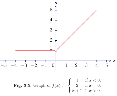
Apart from algebra, a fruitful way to construct new functions is by piecing together known functions. For example, considerf :R→Rdefined by either of the following.
(i)f(x) :=|x|=
x if x≥0,
−x if x <0; (ii)f(x) :=
x+ 2 if x≤1, (x2
−9)/8 if x >1.
The graphs of these functions may be drawn as in Figure 1.4. Taking the integer part or the floor of a real number gives rise to a functionf :R→R
5
1.3 Functions and Their Geometric Properties 21
defined by f(x) := [x], which we refer to as the integer part function or the floor function. Likewise, g : R → R given by g(x) := ⌈x⌉ is called theceiling function. These two functions may also be viewed as examples of functions obtained by piecing together known functions, and their graphs are shown in Figure 1.5. As seen in Figures 1.4 and 1.5, it is often the case that the graphs of functions defined by piecing together different functions look broken or have beak-like edges. Also, in general, such functions are not algebraic. Nevertheless, such functions can be quite useful in constructing examples of certain ‘wild behavior’.
Fig. 1.5. Graphs of the integer part function [x] and the ceiling function ⌈x⌉
Remark 1.14.Polynomials (in one variable) are analogous to integers. Like-wise, rational functions are analogous to rational numbers. Algebraic functions and transcendental functions also have analogues in arithmetic, which are de-fined as follows. A real numberαis called analgebraic numberif it satisfies a nonzero polynomial with integer coefficients. Numbers that are not algebraic are calledtranscendental numbers. For example, it can be easily seen that
√
2,√3,√5
7,√2 +√3 are algebraic numbers. Also, every rational number is an algebraic number. On the other hand, it is not easy to give concrete examples of transcendental numbers. Those interested are referred to the book of Baker [7] for the proof of transcendence of several well-known numbers. ✸
We shall now discuss a number of geometric properties of real-valued func-tions defined on certain subsets ofR.
Bounded Functions
22 1 Numbers and Functions
LetD⊆Randf :D→Rbe a function.
1. f is said to bebounded aboveonDif there isα∈Rsuch thatf(x)≤α for allx∈D. Any suchαis called anupper boundforf.
2. f is said to bebounded belowonDif there isβ∈Rsuch thatf(x)≥β for allx∈D. Any suchβ is called alower boundforf.
3. f is said to be bounded on D if it is bounded above on D and also bounded below onD.
Notice that f is bounded on D if and only if there is γ ∈ R such that
|f(x)| ≤γfor allx∈D. Any suchγis called aboundfor the absolute value of f. Geometrically speaking, f is bounded above means that the graph of f lies below some horizontal line, while f is bounded below means that its graph lies above some horizontal line.
For example,f :R→R defined byf(x) :=−x2 is bounded above on R,
while f : R → R defined by f(x) := x2 is bounded below onR. However,
neither of these functions is bounded on R. On the other hand, f : R →R
defined byf(x) :=x2/(x2+ 1) gives an example of a function that is bounded
onR. For this function, we see readily that 0≤f(x)<1 for all x∈R. The bounds 0 and 1 are, in fact, optimal in the sense that
inf{f(x) :x∈R}= 0 and sup{f(x) :x∈R}= 1.
Of these, the first equality is obvious sincef(x)≥0 for allx∈Randf(0) = 0. To see the second equality, let αbe an upper bound such thatα < 1. Then 1−α >0 and so we can findn∈Nsuch that
1
n <1−α and hence f(
√
n−1) = n−1
n = 1−
1 n > α,
which is a contradiction. This shows that sup{f(x) :x∈R}= 1. Thus there is a qualitative difference between the infimum of (the range of)f, which is attained, and the supremum, which is not attained. This suggests the following general definition.
LetD⊆Randf :D→Rbe a function. We say that
1. f attains its upper boundonD if there isc∈D such that
sup{f(x) :x∈D}=f(c),
2. f attains its lower boundonDif there isd∈D such that
inf{f(x) :x∈D}=f(d),
3. f attains its bounds onD if it attains its upper bound onD and also attains its lower bound onD.
1.3 Functions and Their Geometric Properties 23
Monotonicity, Convexity, and Concavity
Monotonicity is a geometric property of a real-valued function defined on a subset ofRthat corresponds to its graph being increasing or decreasing. For example, consider Figure 1.6, where the graph on the left is increasing while that on the right is decreasing.
a
b
0
x
y
a
b
0
x
y
Fig. 1.6.Typical graphs of increasing and decreasing functions onI= [a, b]
A formal definition is as follows. Let D ⊆Rbe such that D contains an intervalI andf :D→Rbe a function. We say that
1. f is (monotonically)increasingonIif
x1, x2∈I, x1< x2=⇒f(x1)≤f(x2),
2. f is (monotonically)decreasingonI if
x1, x2∈I, x1< x2=⇒f(x1)≥f(x2),
3. f ismonotoniconI iff is monotonically increasing onI orf is mono-tonically decreasing onI.
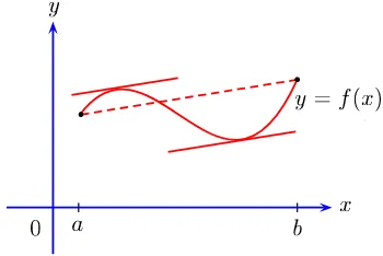
Next, we discuss more subtle properties of a function, known as convexity and concavity. Geometrically, these notions are easily described. A function is convex if the line segment joining any two points on its graph lies on or above the graph. A function is concave if any such line segment lies on or below the graph. An illustration is given in Figure 1.7. To formulate a more precise definition, one should first note that convexity or concavity can be defined relative to an interval I contained in the domain of a function f, and also that given any x1, x2 ∈I withx1 < x2, the equation of the line joining the
corresponding points (x1, f(x1)) and (x2, f(x2)) on the graph off is given by
y−f(x1) =m(x−x1), where m=f(x2)−f(x1)
x2−x1
.
![Fig. 1.7. Typical graphs of convex and concave functions on I = [a, b]](https://thumb-ap.123doks.com/thumbv2/123dok/3935358.1878778/35.441.59.378.53.278/fig-typical-graphs-convex-concave-functions-i-b.webp)