Maria Petrou
Costas Petrou
John Wiley & Sons Ltd, The Atrium, Southern Gate, Chichester, West Sussex, PO19 8SQ, United Kingdom For details of our global editorial offices, for customer services and for information about how to apply for permission to reuse the copyright material in this book please see our website at www.wiley.com.
The right of the author to be identified as the author of this work has been asserted in accordance with the Copyright, Designs and Patents Act 1988.
All rights reserved. No part of this publication may be reproduced, stored in a retrieval system, or transmitted, in any form or by any means, electronic, mechanical, photocopying, recording or otherwise, except as permitted by the UK Copyright, Designs and Patents Act 1988, without the prior permission of the publisher.
Wiley also publishes its books in a variety of electronic formats. Some content that appears in print may not be available in electronic books.
Designations used by companies to distinguish their products are often claimed as trademarks. All brand names and product names used in this book are trade names, service marks, trademarks or registered trademarks of their respective owners. The publisher is not associated with any product or vendor mentioned in this book. This publication is designed to provide accurate and authoritative information in regard to the subject matter covered. It is sold on the understanding that the publisher is not engaged in rendering professional services. If professional advice or other expert assistance is required, the services of a competent professional should be sought.
Library of Congress Cataloging-in-Publication Data Petrou, Maria.
Image processing : the fundamentals / Maria Petrou, Costas Petrou. – 2nd ed. p. cm.
Includes bibliographical references and index. ISBN 978-0-470-74586-1 (cloth)
1. Image processing – Digital techniques. TA1637.P48 2010
621.36′7 – dc22
2009053150 ISBN 978-0-470-74586-1
Preface xxiii
1 Introduction 1
Why do we process images? . . . 1
What is an image? . . . 1
What is a digital image? . . . 1
What is a spectral band? . . . 2
Why do most image processing algorithms refer to grey images, while most images we come across are colour images? . . . 2
How is a digital image formed? . . . 3
If a sensor corresponds to a patch in the physical world, how come we can have more than one sensor type corresponding to the same patch of the scene? . . . 3
What is the physical meaning of the brightness of an image at a pixel position? . . 3
Why are images often quoted as being 512×512, 256×256, 128×128 etc? . . . . 6
How many bits do we need to store an image? . . . 6
What determines the quality of an image? . . . 7
What makes an image blurred? . . . 7
What is meant by image resolution? . . . 7
What does “good contrast” mean? . . . 10
What is the purpose of image processing? . . . 11
How do we do image processing? . . . 11
Do we use nonlinear operators in image processing? . . . 12
What is a linear operator? . . . 12
How are linear operators defined? . . . 12
What is the relationship between the point spread function of an imaging device and that of a linear operator? . . . 12
How does a linear operator transform an image? . . . 12
What is the meaning of the point spread function? . . . 13
Box 1.1. The formal definition of a point source in the continuous domain . . . 14
How can we express in practice the effect of a linear operator on an image? . . . . 18
Can we apply more than one linear operators to an image? . . . 22
Does the order by which we apply the linear operators make any difference to the result? . . . 22
Box 1.3. What is the stacking operator? . . . 29
What is the implication of the separability assumption on the structure of matrixH? 38 How can a separable transform be written in matrix form? . . . 39
What is the meaning of the separability assumption? . . . 40
Box 1.4. The formal derivation of the separable matrix equation . . . 41
What is the “take home” message of this chapter? . . . 43
What is the significance of equation (1.108) in linear image processing? . . . 43
What is this book about? . . . 44
2 Image Transformations 47 What is this chapter about? . . . 47
How can we define an elementary image? . . . 47
What is the outer product of two vectors? . . . 47
How can we expand an image in terms of vector outer products? . . . 47
How do we choose matriceshc andhr? . . . 49
What is a unitary matrix? . . . 50
What is the inverse of a unitary transform? . . . 50
How can we construct a unitary matrix? . . . 50
How should we choose matricesU andV so thatgcan be represented by fewer bits thanf? . . . 50
What is matrix diagonalisation? . . . 50
Can we diagonalise any matrix? . . . 50
2.1 Singular value decomposition . . . 51
How can we diagonalise an image? . . . 51
Box 2.1. Can we expand in vector outer products any image? . . . 54
How can we compute matricesU,V and Λ12 needed for image diagonalisation? . . 56
Box 2.2. What happens if the eigenvalues of matrixggT are negative? . . . 56
What is the singular value decomposition of an image? . . . 60
Can we analyse an eigenimage into eigenimages? . . . 61
How can we approximate an image using SVD? . . . 62
Box 2.3. What is the intuitive explanation of SVD? . . . 62
What is the error of the approximation of an image by SVD? . . . 63
How can we minimise the error of the reconstruction? . . . 65
Are there any sets of elementary images in terms of whichanyimage may be expanded? 72 What is a complete and orthonormal set of functions? . . . 72
Are there any complete sets of orthonormal discrete valued functions? . . . 73
2.2 Haar, Walsh and Hadamard transforms . . . 74
How are the Haar functions defined? . . . 74
How are the Walsh functions defined? . . . 74
Box 2.4. Definition of Walsh functions in terms of the Rademacher functions . . . 74
How can we use the Haar or Walsh functions to create image bases? . . . 75
How can we create the image transformation matrices from the Haar and Walsh functions in practice? . . . 76
What do the elementary images of the Haar transform look like? . . . 80
Can we define an orthogonal matrix with entries only +1 or−1? . . . 85
Box 2.5. Ways of ordering the Walsh functions . . . 86
What are the advantages and disadvantages of the Walsh and the Haar transforms? 92
What is the Haar wavelet? . . . 93
2.3 Discrete Fourier transform . . . 94
What is the discrete version of the Fourier transform (DFT)? . . . 94
Box 2.6. What is the inverse discrete Fourier transform? . . . 95
How can we write the discrete Fourier transform in a matrix form? . . . 96
Is matrixU used for DFT unitary? . . . 99
Which are the elementary images in terms of which DFT expands an image? . . . 101
Why is the discrete Fourier transform more commonly used than the other transforms? . . . 105
What does the convolution theorem state? . . . 105
Box 2.7. If a function is the convolution of two other functions, what is the rela-tionship of its DFT with the DFTs of the two functions? . . . 105
How can we display the discrete Fourier transform of an image? . . . 112
What happens to the discrete Fourier transform of an image if the image is rotated? . . . 113
What happens to the discrete Fourier transform of an image if the image is shifted? . . . 114
What is the relationship between the average value of the image and its DFT? . . 118
What happens to the DFT of an image if the image is scaled? . . . 119
Box 2.8. What is the Fast Fourier Transform? . . . 124
What are the advantages and disadvantages of DFT? . . . 126
Can we have a real valued DFT? . . . 126
Can we have a purely imaginary DFT? . . . 130
Can an image have a purely real or a purely imaginary valued DFT? . . . 137
2.4 The even symmetric discrete cosine transform (EDCT) . . . 138
What is the even symmetric discrete cosine transform? . . . 138
Box 2.9. Derivation of the inverse 1D even discrete cosine transform . . . 143
What is the inverse 2D even cosine transform? . . . 145
What are the basis images in terms of which the even cosine transform expands an image? . . . 146
2.5 The odd symmetric discrete cosine transform (ODCT) . . . 149
What is the odd symmetric discrete cosine transform? . . . 149
Box 2.10. Derivation of the inverse 1D odd discrete cosine transform . . . 152
What is the inverse 2D odd discrete cosine transform? . . . 154
What are the basis images in terms of which the odd discrete cosine transform expands an image? . . . 154
2.6 The even antisymmetric discrete sine transform (EDST) . . . 157
What is the even antisymmetric discrete sine transform? . . . 157
Box 2.11. Derivation of the inverse 1D even discrete sine transform . . . 160
What is the inverse 2D even sine transform? . . . 162
What are the basis images in terms of which the even sine transform expands an image? . . . 163
What happens if we do not remove the mean of the image before we compute its EDST? . . . 166
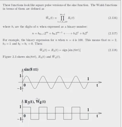
2.7 The odd antisymmetric discrete sine transform (ODST) . . . 167
Box 2.12. Derivation of the inverse 1D odd discrete sine transform . . . 171
What is the inverse 2D odd sine transform? . . . 172
What are the basis images in terms of which the odd sine transform expands an image? . . . 173
What is the “take home” message of this chapter? . . . 176
3 Statistical Description of Images 177 What is this chapter about? . . . 177
Why do we need the statistical description of images? . . . 177
3.1 Random fields . . . 178
What is a random field? . . . 178
What is a random variable? . . . 178
What is a random experiment? . . . 178
How do we perform a random experiment with computers? . . . 178
How do we describe random variables? . . . 178
What is the probability of an event? . . . 179
What is the distribution function of a random variable? . . . 180
What is the probability of a random variable taking a specific value? . . . 181
What is the probability density function of a random variable? . . . 181
How do we describe many random variables? . . . 184
What relationships maynrandom variables have with each other? . . . 184
How do we define a random field? . . . 189
How can we relate two random variables that appear in the same random field? . . 190
How can we relate two random variables that belong to two different random fields? . . . 193
If we have just one image from an ensemble of images, can we calculate expectation values? . . . 195
When is a random field homogeneous with respect to the mean? . . . 195
When is a random field homogeneous with respect to the autocorrelation function? 195 How can we calculate the spatial statistics of a random field? . . . 196
How do we compute the spatial autocorrelation function of an image in practice? . 196 When is a random field ergodic with respect to the mean? . . . 197
When is a random field ergodic with respect to the autocorrelation function? . . . 197
What is the implication of ergodicity? . . . 199
Box 3.1. Ergodicity, fuzzy logic and probability theory . . . 200
How can we construct a basis of elementary images appropriate for expressing in an optimal way a whole set of images? . . . 200
3.2 Karhunen-Loeve transform . . . 201
What is the Karhunen-Loeve transform? . . . 201
Why does diagonalisation of the autocovariance matrix of a set of images define a desirable basis for expressing the images in the set? . . . 201
How can we transform an image so its autocovariance matrix becomes diagonal? . 204 What is the form of the ensemble autocorrelation matrix of a set of images, if the ensemble is stationary with respect to the autocorrelation? . . . 210
How do we go from the 1D autocorrelation function of the vector representation of an image to its 2D autocorrelation matrix? . . . 211
How do we compute the K-L transform of an image in practice? . . . 214
How do we compute the Karhunen-Loeve (K-L) transform of an ensemble of images? . . . 215
Is the assumption of ergodicity realistic? . . . 215
Box 3.2. How can we calculate the spatial autocorrelation matrix of an image, when it is represented by a vector? . . . 215
Is the mean of the transformed image expected to be really 0? . . . 220
How can we approximate an image using its K-L transform? . . . 220
What is the error with which we approximate an image when we truncate its K-L expansion? . . . 220
What are the basis images in terms of which the Karhunen-Loeve transform expands an image? . . . 221
Box 3.3. What is the error of the approximation of an image using the Karhunen-Loeve transform? . . . 226
3.3 Independent component analysis . . . 234
What is Independent Component Analysis (ICA)? . . . 234
What is the cocktail party problem? . . . 234
How do we solve the cocktail party problem? . . . 235
What does the central limit theorem say? . . . 235
What do we mean by saying that “the samples of x1(t) are more Gaussianly dis-tributed than either s1(t) or s2(t)” in relation to the cocktail party problem? Are we talking about the temporalsamples of x1(t), or are we talking about all possible versions ofx1(t) at a given time? . . . 235
How do we measure non-Gaussianity? . . . 239
How are the moments of a random variable computed? . . . 239
How is the kurtosis defined? . . . 240
How is negentropy defined? . . . 243
How is entropy defined? . . . 243
Box 3.4. From all probability density functions with the same variance, the Gaussian has the maximum entropy . . . 246
How is negentropy computed? . . . 246
Box 3.5. Derivation of the approximation of negentropy in terms of moments . . . 252
Box 3.6. Approximating the negentropy with nonquadratic functions . . . 254
Box 3.7. Selecting the nonquadratic functions with which to approximate the ne-gentropy . . . 257
How do we apply the central limit theorem to solve the cocktail party problem? . . 264
How may ICA be used in image processing? . . . 264
How do we search for the independent components? . . . 264
How can we whiten the data? . . . 266
How can we select the independent components from whitened data? . . . 267
Box 3.8. How does the method of Lagrange multipliers work? . . . 268
Box 3.9. How can we choose a direction that maximises the negentropy? . . . 269
How do we perform ICA in image processing in practice? . . . 274
How do we apply ICA to signal processing? . . . 283
What are the major characteristics of independent component analysis? . . . 289
4 Image Enhancement 293
What is image enhancement? . . . 293
How can we enhance an image? . . . 293
What is linear filtering? . . . 293
4.1 Elements of linear filter theory. . . 294
How do we define a 2D filter? . . . 294
How are the frequency response function and the unit sample response of the filter related? . . . 294
Why are we interested in the filter function in the real domain? . . . 294
Are there any conditions whichh(k, l) must fulfil so that it can be used as a convo-lution filter? . . . 294
Box 4.1. What is the unit sample response of the 2D ideal low pass filter? . . . 296
What is the relationship between the 1D and the 2D ideal lowpass filters? . . . 300
How can we implement in the real domain a filter that is infinite in extent? . . . . 301
Box 4.2. z-transforms . . . 301
Can we define a filter directly in the real domain for convenience? . . . 309
Can we define a filter in the real domain, without side lobes in the frequency domain? . . . 309
4.2 Reducing high frequency noise . . . 311
What are the types of noise present in an image? . . . 311
What is impulse noise? . . . 311
What is Gaussian noise? . . . 311
What is additive noise? . . . 311
What is multiplicative noise? . . . 311
What is homogeneous noise? . . . 311
What is zero-mean noise? . . . 312
What is biased noise? . . . 312
What is independent noise? . . . 312
What is uncorrelated noise? . . . 312
What is white noise? . . . 313
What is the relationship between zero-mean uncorrelated and white noise? . . . . 313
What is iid noise? . . . 313
Is it possible to have white noise that is not iid? . . . 315
Box 4.3. The probability density function of a function of a random variable . . . 320
Why is noise usually associated with high frequencies? . . . 324
How do we deal with multiplicative noise? . . . 325
Box 4.4. The Fourier transform of the delta function . . . 325
Box 4.5. Wiener-Khinchine theorem . . . 325
Is the assumption of Gaussian noise in an image justified? . . . 326
How do we remove shot noise? . . . 326
What is a rank order filter? . . . 326
What is median filtering? . . . 326
What is mode filtering? . . . 328
How do we reduce Gaussian noise? . . . 328
Can we have weighted median and mode filters like we have weighted mean filters? 333 Can we filter an image by using the linear methods we learnt in Chapter 2? . . . . 335
Can we avoid blurring the image when we are smoothing it? . . . 337
What is the edge adaptive smoothing? . . . 337
Box 4.6. Efficient computation of the local variance . . . 339
How does the mean shift algorithm work? . . . 339
What is anisotropic diffusion? . . . 342
Box 4.7. Scale space and the heat equation . . . 342
Box 4.8. Gradient, Divergence and Laplacian . . . 345
Box 4.9. Differentiation of an integral with respect to a parameter . . . 348
Box 4.10. From the heat equation to the anisotropic diffusion algorithm . . . 348
How do we perform anisotropic diffusion in practice? . . . 349
4.3 Reducing low frequency interference . . . 351
When does low frequency interference arise? . . . 351
Can variable illumination manifest itself in high frequencies? . . . 351
In which other cases may we be interested in reducing low frequencies? . . . 351
What is the ideal high pass filter? . . . 351
How can we enhance small image details using nonlinear filters? . . . 357
What is unsharp masking? . . . 357
How can we apply the unsharp masking algorithm locally? . . . 357
How does the locally adaptive unsharp masking work? . . . 358
How does the retinex algorithm work? . . . 360
Box 4.11. Which are the grey values that are stretched most by the retinex algorithm? . . . 360
How can we improve an image which suffers from variable illumination? . . . 364
What is homomorphic filtering? . . . 364
What is photometric stereo? . . . 366
What does flatfielding mean? . . . 366
How is flatfielding performed? . . . 366
4.4 Histogram manipulation . . . 367
What is the histogram of an image? . . . 367
When is it necessary to modify the histogram of an image? . . . 367
How can we modify the histogram of an image? . . . 367
What is histogram manipulation? . . . 368
What affects the semantic information content of an image? . . . 368
How can we perform histogram manipulation and at the same time preserve the information content of the image? . . . 368
What is histogram equalisation? . . . 370
Why do histogram equalisation programs usually not produce images with flat his-tograms? . . . 370
How do we perform histogram equalisation in practice? . . . 370
Can we obtain an image with a perfectly flat histogram? . . . 372
What if we do not wish to have an image with a flat histogram? . . . 373
How do we do histogram hyperbolisation in practice? . . . 373
How do we do histogram hyperbolisation with random additions? . . . 374
Why should one wish to perform something other than histogram equalisation? . . 374
What if the image has inhomogeneous contrast? . . . 375
How can we enhance an image by stretching only the grey values that appear in
genuine brightness transitions? . . . 377
How do we perform pairwise image enhancement in practice? . . . 378
4.5 Generic deblurring algorithms . . . 383
How does mode filtering help deblur an image? . . . 383
Can we use an edge adaptive window to apply the mode filter? . . . 385
How can mean shift be used as a generic deblurring algorithm? . . . 385
What is toboggan contrast enhancement? . . . 387
How do we do toboggan contrast enhancement in practice? . . . 387
What is the “take home” message of this chapter? . . . 393
5 Image Restoration 395 What is image restoration? . . . 395
Why may an image require restoration? . . . 395
What is image registration? . . . 395
How is image restoration performed? . . . 395
What is the difference between image enhancement and image restoration? . . . . 395
5.1 Homogeneous linear image restoration: inverse filtering. . . 396
How do we model homogeneous linear image degradation? . . . 396
How may the problem of image restoration be solved? . . . 396
How may we obtain information on the frequency response function ˆH(u, v) of the degradation process? . . . 396
If we know the frequency response function of the degradation process, isn’t the solution to the problem of image restoration trivial? . . . 407
What happens at frequencies where the frequency response function is zero? . . . . 408
Will the zeros of the frequency response function and the image always coincide? . . . 408
How can we avoid the amplification of noise? . . . 408
How do we apply inverse filtering in practice? . . . 410
Can we define a filter that will automatically take into consideration the noise in the blurred image? . . . 417
5.2 Homogeneous linear image restoration: Wiener filtering . . . 419
How can we express the problem of image restoration as a least square error esti-mation problem? . . . 419
Can we find a linear least squares error solution to the problem of image restoration? . . . 419
What is the linear least mean square error solution of the image restoration problem? . . . 420
Box 5.1. The least squares error solution . . . 420
Box 5.2. From the Fourier transform of the correlation functions of images to their spectral densities . . . 427
Box 5.3. Derivation of the Wiener filter . . . 428
What is the relationship between Wiener filtering and inverse filtering? . . . 430
How can we determine the spectral density of the noise field? . . . 430
How can we possibly use Wiener filtering, if we know nothing about the statistical properties of the unknown image? . . . 430
5.3 Homogeneous linear image restoration: Constrained matrix inversion436 If the degradation process is assumed linear, why don’t we solve a system of linear
equations to reverse its effect instead of invoking the convolution theorem? . 436 Equation (5.146) seems pretty straightforward, why bother with any other
approach? . . . 436
Is there any way by which matrixH can be inverted? . . . 437
When is a matrix block circulant? . . . 437
When is a matrix circulant? . . . 438
Why can block circulant matrices be inverted easily? . . . 438
Which are the eigenvalues and eigenvectors of a circulant matrix? . . . 438
How does the knowledge of the eigenvalues and the eigenvectors of a matrix help in inverting the matrix? . . . 439
How do we know that matrix H that expresses the linear degradation process is block circulant? . . . 444
How can we diagonalise a block circulant matrix? . . . 445
Box 5.4. Proof of equation (5.189) . . . 446
Box 5.5. What is the transpose of matrix H? . . . 448
How can we overcome the extreme sensitivity of matrix inversion to noise? . . . 455
How can we incorporate the constraint in the inversion of the matrix? . . . 456
Box 5.6. Derivation of the constrained matrix inversion filter . . . 459
What is the relationship between the Wiener filter and the constrained matrix in-version filter? . . . 462
How do we apply constrained matrix inversion in practice? . . . 464
5.4 Inhomogeneous linear image restoration: the whirl transform . . . . 468
How do we model the degradation of an image if it is linear but inhomogeneous? . 468 How may we use constrained matrix inversion when the distortion matrix is not circulant? . . . 477
What happens if matrixH is really very big and we cannot take its inverse? . . . . 481
Box 5.7. Jacobi’s method for inverting large systems of linear equations . . . 482
Box 5.8. Gauss-Seidel method for inverting large systems of linear equations . . . . 485
Does matrixH as constructed in examples 5.41, 5.43, 5.44 and 5.45 fulfil the condi-tions for using the Gauss-Seidel or the Jacobi method? . . . 485
What happens if matrix H does not satisfy the conditions for the Gauss-Seidel method? . . . 486
How do we apply the gradient descent algorithm in practice? . . . 487
What happens if we do not know matrixH? . . . 489
5.5 Nonlinear image restoration: MAP estimation. . . 490
What does MAP estimation mean? . . . 490
How do we formulate the problem of image restoration as a MAP estimation? . . . 490
How do we select the most probable configuration of restored pixel values, given the degradation model and the degraded image? . . . 490
Box 5.9. Probabilities: prior, a priori, posterior, a posteriori, conditional . . . 491
Is the minimum of the cost function unique? . . . 491
How can we select then one solution from all possible solutions that minimise the cost function? . . . 493
Can we combine the posterior and the prior probabilities for a configurationx? . . 493
How do we model in general the cost function we have to minimise in order to restore
an image? . . . 499
What is the reason we use a temperature parameter when we model the joint prob-ability density function, since its does not change the configuration for which the probability takes its maximum? . . . 501
How does the temperature parameter allow us to focus or defocus in the solution space? . . . 501
How do we model the prior probabilities of configurations? . . . 501
What happens if the image has genuine discontinuities? . . . 502
How do we minimise the cost function? . . . 503
How do we create a possible new solution from the previous one? . . . 503
How do we know when to stop the iterations? . . . 505
How do we reduce the temperature in simulated annealing? . . . 506
How do we perform simulated annealing with the Metropolis sampler in practice? . 506 How do we perform simulated annealing with the Gibbs sampler in practice? . . . 507
Box 5.11. How can we draw random numbers according to a given probability density function? . . . 508
Why is simulated annealing slow? . . . 511
How can we accelerate simulated annealing? . . . 511
How can we coarsen the configuration space? . . . 512
5.6 Geometric image restoration . . . 513
How may geometric distortion arise? . . . 513
Why do lenses cause distortions? . . . 513
How can a geometrically distorted image be restored? . . . 513
How do we perform the spatial transformation? . . . 513
How may we model the lens distortions? . . . 514
How can we model the inhomogeneous distortion? . . . 515
How can we specify the parameters of the spatial transformation model? . . . 516
Why is grey level interpolation needed? . . . 516
Box 5.12. The Hough transform for line detection . . . 520
What is the “take home” message of this chapter? . . . 526
6 Image Segmentation and Edge Detection 527 What is this chapter about? . . . 527
What exactly is the purpose of image segmentation and edge detection? . . . 527
6.1 Image segmentation. . . 528
How can we divide an image into uniform regions? . . . 528
What do we mean by “labelling” an image? . . . 528
What can we do if the valley in the histogram is not very sharply defined? . . . 528
How can we minimise the number of misclassified pixels? . . . 529
How can we choose the minimum error threshold? . . . 530
What is the minimum error threshold when object and background pixels are nor-mally distributed? . . . 534
What is the meaning of the two solutions of the minimum error threshold equation? . . . 535
What are the drawbacks of the minimum error threshold method? . . . 541
Is there any method that does not depend on the availability of models for the distributions of the object and the background pixels? . . . 541
Box 6.1. Derivation of Otsu’s threshold . . . 542
Are there any drawbacks in Otsu’s method? . . . 545
How can we threshold images obtained under variable illumination? . . . 545
If we threshold the image according to the histogram of lnf(x, y), are we thresholding it according to the reflectance properties of the imaged surfaces? . . . 545
Box 6.2. The probability density function of the sum of two random variables . . . 546
Since straightforward thresholding methods break down under variable illumination, how can we cope with it? . . . 548
What do we do if the histogram has only one peak? . . . 549
Are there any shortcomings of the grey value thresholding methods? . . . 550
How can we cope with images that contain regions that are not uniform but they areperceivedas uniform? . . . 551
Can we improve histogramming methods by taking into consideration the spatial proximity of pixels? . . . 553
Are there any segmentation methods that take into consideration the spatial prox-imity of pixels? . . . 553
How can one choose the seed pixels? . . . 554
How does the split and merge method work? . . . 554
What is morphological image reconstruction? . . . 554
How does morphological image reconstruction allow us to identify the seeds needed for the watershed algorithm? . . . 557
How do we compute the gradient magnitude image? . . . 557
What is the role of the number we subtract fromf to create maskgin the morpho-logical reconstruction off byg? . . . 558
What is the role of the shape and size of the structuring element in the morphological reconstruction off byg? . . . 560
How does the use of the gradient magnitude image help segment the image by the watershed algorithm? . . . 566
Are there any drawbacks in the watershed algorithm which works with the gradient magnitude image? . . . 568
Is it possible to segment an image by filtering? . . . 574
How can we use the mean shift algorithm to segment an image? . . . 574
What is a graph? . . . 576
How can we use a graph to represent an image? . . . 576
How can we use the graph representation of an image to segment it? . . . 576
What is the normalised cuts algorithm? . . . 576
Box 6.3. The normalised cuts algorithm as an eigenvalue problem . . . 576
Box 6.4. How do we minimise the Rayleigh quotient? . . . 585
How do we apply the normalised graph cuts algorithm in practice? . . . 589
Is it possible to segment an image by considering thedissimilaritiesbetween regions, as opposed to considering the similarities between pixels? . . . 589
6.2 Edge detection . . . 591
What is the smallest possible window we can choose? . . . 592
What happens when the image has noise? . . . 593
Box 6.5. How can we choose the weights of a 3×3 mask for edge detection? . . . . 595
What is the best value of parameterK? . . . 596
Box 6.6. Derivation of the Sobel filters . . . 596
In the general case, how do we decide whether a pixel is an edge pixel or not? . . . 601
How do we perform linear edge detection in practice? . . . 602
Are Sobel masks appropriate for all images? . . . 605
How can we choose the weights of the mask if we need a larger mask owing to the presence of significant noise in the image? . . . 606
Can we use the optimal filters for edges to detect lines in an image in an optimal way? . . . 609
What is the fundamental difference between step edges and lines? . . . 609
Box 6.7. Convolving a random noise signal with a filter . . . 615
Box 6.8. Calculation of the signal to noise ratio after convolution of a noisy edge signal with a filter . . . 616
Box 6.9. Derivation of the good locality measure . . . 617
Box 6.10. Derivation of the count of false maxima . . . 619
Can edge detection lead to image segmentation? . . . 620
What is hysteresis edge linking? . . . 621
Does hysteresis edge linking lead to closed edge contours? . . . 621
What is the Laplacian of Gaussian edge detection method? . . . 623
Is it possible to detect edges and lines simultaneously? . . . 623
6.3 Phase congruency and the monogenic signal . . . 625
What is phase congruency? . . . 625
What is phase congruency for a 1D digital signal? . . . 625
How does phase congruency allow us to detect lines and edges? . . . 626
Why does phase congruency coincide with the maximum of the local energy of the signal? . . . 626
How can we measure phase congruency? . . . 627
Couldn’t we measure phase congruency by simply averaging the phases of the har-monic components? . . . 627
How do we measure phase congruency in practice? . . . 630
How do we measure the local energy of the signal? . . . 630
Why should we perform convolution with the two basis signals in order to get the projection of the local signal on the basis signals? . . . 632
Box 6.11. Some properties of the continuous Fourier transform . . . 637
If all we need to compute is the local energy of the signal, why don’t we use Parseval’s theorem to compute it in the real domain inside a local window? . . . 647
How do we decide which filters to use for the calculation of the local energy? . . . 648
How do we compute the local energy of a 1D signal in practice? . . . 651
How can we tell whether the maximum of the local energy corresponds to a sym-metric or an antisymsym-metric feature? . . . 652
How can we compute phase congruency and local energy in 2D? . . . 659
What is the analytic signal? . . . 659
How can we generalise the Hilbert transform to 2D? . . . 660
How can the monogenic signal be used? . . . 660
How do we select the even filter we use? . . . 661
What is the “take home” message of this chapter? . . . 668
7 Image Processing for Multispectral Images 669 What is a multispectral image? . . . 669
What are the problems that are special to multispectral images? . . . 669
What is this chapter about? . . . 670
7.1 Image preprocessing for multispectral images . . . 671
Why may one wish to replace the bands of a multispectral image with other bands? . . . 671
How do we usually construct a grey image from a multispectral image? . . . 671
How can we construct a single band from a multispectral image that contains the maximum amount of image information? . . . 671
What is principal component analysis? . . . 672
Box 7.1. How do we measure information? . . . 673
How do we perform principal component analysis in practice? . . . 674
What are the advantages of using the principal components of an image, instead of the original bands? . . . 675
What are the disadvantages of using the principal components of an image instead of the original bands? . . . 675
Is it possible to work out only the first principal component of a multispectral image if we are not interested in the other components? . . . 682
Box 7.2. The power method for estimating the largest eigenvalue of a matrix . . . 682
What is the problem of spectral constancy? . . . 684
What influences the spectral signature of a pixel? . . . 684
What is the reflectance function? . . . 684
Does the imaging geometry influence the spectral signature of a pixel? . . . 684
How does the imaging geometry influence the light energy a pixel receives? . . . . 685
How do we model the process of image formation for Lambertian surfaces? . . . . 685
How can we eliminate the dependence of the spectrum of a pixel on the imaging geometry? . . . 686
How can we eliminate the dependence of the spectrum of a pixel on the spectrum of the illuminating source? . . . 686
What happens if we have more than one illuminating sources? . . . 687
How can we remove the dependence of the spectral signature of a pixel on the imaging geometry and on the spectrum of the illuminant? . . . 687
What do we have to do if the imaged surface is not made up from the same material? . . . 688
What is the spectral unmixing problem? . . . 688
How do we solve the linear spectral unmixing problem? . . . 689
Can we use library spectra for the pure materials? . . . 689
How do we solve the linear spectral unmixing problem when we know the spectra of the pure components? . . . 690
Is it possible that the inverse of matrixQcannot be computed? . . . 693
What happens if we do not know which pure substances might be present in the
mixed substance? . . . 694
How do we solve the linear spectral unmixing problem if we do not know the spectra of the pure materials? . . . 695
7.2 The physics and psychophysics of colour vision . . . 700
What is colour? . . . 700
What is the interest in colour from the engineering point of view? . . . 700
What influences the colour we perceive for a dark object? . . . 700
What causes the variations of the daylight? . . . 701
How can we model the variations of the daylight? . . . 702
Box 7.3. Standard illuminants . . . 704
What is the observed variation in the natural materials? . . . 706
What happens to the light once it reaches the sensors? . . . 711
Is it possible for different materials to produce the same recording by a sensor? . . 713
How does the human visual system achieve colour constancy? . . . 714
What does the trichromatic theory of colour vision say? . . . 715
What defines a colour system? . . . 715
How are the tristimulus values specified? . . . 715
Can all monochromatic reference stimuli be matched by simply adjusting the inten-sities of the primary lights? . . . 715
Do all people require the same intensities of the primary lights to match the same monochromatic reference stimulus? . . . 717
Who are the people with normal colour vision? . . . 717
What are the most commonly used colour systems? . . . 717
What is theCIE RGB colour system? . . . 717
What is theXY Z colour system? . . . 718
How do we represent colours in 3D? . . . 718
How do we represent colours in 2D? . . . 718
What is the chromaticity diagram? . . . 719
Box 7.4. Some useful theorems from 3D geometry . . . 721
What is the chromaticity diagram for theCIE RGBcolour system? . . . 724
How does the human brain perceive colour brightness? . . . 725
How is the alychne defined in theCIE RGBcolour system? . . . 726
How is theXY Z colour system defined? . . . 726
What is the chromaticity diagram of theXY Z colour system? . . . 728
How is it possible to create a colour system with imaginary primaries, in practice? 729 What if we wish to model the way a particular individual sees colours? . . . 729
If different viewers require different intensities of the primary lights to see white, how do we calibrate colours between different viewers? . . . 730
How do we make use of the reference white? . . . 730
How is thesRGB colour system defined? . . . 732
Does a colour change if we double all its tristimulus values? . . . 733
How does the description of a colour, in terms of a colour system, relate to the way we describe colours in everyday language? . . . 733
How do we compare colours? . . . 733
What is a metric? . . . 733
Which are the perceptually uniform colour spaces? . . . 734
How is theLuvcolour space defined? . . . 734
How is theLabcolour space defined? . . . 735
How do we choose values for (Xn, Yn, Zn)? . . . 735
How can we compute theRGB values from theLuv values? . . . 735
How can we compute theRGB values from theLabvalues? . . . 736
How do we measure perceived saturation? . . . 737
How do we measure perceived differences in saturation? . . . 737
How do we measure perceived hue? . . . 737
How is the perceived hue angle defined? . . . 738
How do we measure perceived differences in hue? . . . 738
What affects the way we perceive colour? . . . 740
What is meant by temporal context of colour? . . . 740
What is meant by spatial context of colour? . . . 740
Why distance matters when we talk about spatial frequency? . . . 741
How do we explain the spatial dependence of colour perception? . . . 741
7.3 Colour image processing in practice . . . 742
How does the study of the human colour vision affect the way we do image processing? . . . 742
How perceptually uniform are the perceptually uniform colour spaces in practice? . 742 How should we convert the imageRGB values to theLuv or theLabcolour spaces? . . . 742
How do we measure hue and saturation in image processing applications? . . . 747
How can we emulate the spatial dependence of colour perception in image processing? . . . 752
What is the relevance of the phenomenon of metamerism to image processing? . . 756
How do we cope with the problem of metamerism in an industrial inspection appli-cation? . . . 756
What is a Monte-Carlo method? . . . 757
How do we remove noise from multispectral images? . . . 759
How do we rank vectors? . . . 760
How do we deal with mixed noise in multispectral images? . . . 760
How do we enhance a colour image? . . . 761
How do we restore multispectral images? . . . 767
How do we compress colour images? . . . 767
How do we segment multispectral images? . . . 767
How do we applyk-means clustering in practice? . . . 767
How do we extract the edges of multispectral images? . . . 769
What is the “take home” message of this chapter? . . . 770
Bibliographical notes 775
References 777
Since the first edition of this book in 1999, the field of Image Processing has seen many developments. First of all, the proliferation of colour sensors caused an explosion of research in colour vision and colour image processing. Second, application of image processing to biomedicine has really taken off, with medical image processing nowadays being almost a field of its own. Third, image processing has become more sophisticated, having reached out even further afield, into other areas of research, as diverse as graph theory and psychophysics, to borrow methodologies and approaches.
This new edition of the book attempts to capture these new insights, without, however, forgetting the well known and established methods of image processing of the past. The book may be treated as three books interlaced: the advanced proofs and peripheral material are presented in grey boxes; they may be omitted in a first reading or for an undergraduate course. The back bone of the book is the text given in the form of questions and answers. We believe that the order of the questions is that of coming naturally to the reader when they encounter a new concept. There are 255 figures and 384 fully worked out examples aimed at clarifying these concepts. Examples with a number prefixed with a “B” refer to the boxed material and again they may be omitted in a first reading or an undergraduate course. The book is accompanied by a CD with all the MatLab programs that produced the examples and the figures. There is also a collection of slide presentations in pdf format, available from the accompanying web page of the book, that may help the lecturer who wishes to use this material for teaching.
We have made a great effort to make the book easy to read and we hope that learning about the “nuts and bolts” behind the image processing algorithms will make the subject even more exciting and a pleasure to delve into.
Over the years of writing this book, we were helped by various people. We would par-ticularly like to thank Mike Brookes, Nikos Mitianoudis, Antonis Katartzis, Mohammad Ja-hangiri, Tania Stathaki and Vladimir Jeliazkov, for useful discussions, Mohammad JaJa-hangiri, Leila Favaedi and Olga Duran for help with some figures, and Pedro Garcia-Sevilla for help with typesetting the book.
(a) (b)
Plate I: (a) The colours of the Macbeth colour chart. (b) The chromaticity diagram of the XY Z colour system. Points A andB represent colours which, although further apart than pointsC andD, are perceived as more similar than the colours represented byC andD.
(a) One eigenvalue (b) Two eigenvalues (c) Three eigenvalues
(d) Four eigenvalues (e) Five eigenvalues (f) Six eigenvalues
Plate II: The inclusion of extra eigenvalues beyond the third one changes the colour appear-ance very little (see example 7.12, on page 713).
Plate IV: Colour perception depends on colour context (see page 740).
(a) 5% impulse noise (b) 5% impulse + Gaussian (σ= 15)
(a) Original (b) Seen from 2m
(c) Seen from 4m (d) Seen from 6m
Plate VI: (a) “A Street in Shanghai” (344×512). As seen from (b) 2m, (c) 4m and (d) 10m distance. In (b) a border of 10 pixels around should be ignored, in (c) the stripe affected by border effects is 22 pixels wide, while in (d) is 34 pixels wide (example 7.28, page 754).
(a) “Abu-Dhabi building” (b) After colour enhancement
(a) “Vina del Mar-Valparaiso” (b) After colour enhancement
Plate VIII: Enhancing colours by increasing their saturation to the maximum, while retaining their hue. Threshold= 0.01 andγ= 1/√6 were used for the saturation (see page 761).
(a) Original (184×256) (b) 10-means (sRGB)
(c) Mean shift (sRGB) (d) Mean shift (CIE RGB)
Plate IX: “The Merchant in Al-Ain” segmented in Luv space, assuming that the original values are either in theCIE RGB or thesRGB space (see example 7.37, on page 768).
Introduction
Why do we process images?
Image Processing has been developed in response to three major problems concerned with pictures:
• picture digitisation and coding to facilitate transmission, printing and storage of pic-tures;
• picture enhancement and restoration in order, for example, to interpret more easily pictures of the surface of other planets taken by various probes;
• picture segmentation and description as an early stage to Machine Vision.
Image Processing nowadays refers mainly to the processing of digital images.
What is an image?
Apanchromatic imageis a 2D light intensity function, f(x, y), where xand y are spatial coordinates and the value off at (x, y) is proportional to the brightness of the scene at that point. If we have a multispectral image, f(x, y) is a vector, each component of which indicates the brightness of the scene at point (x, y) at the corresponding spectralband.
What is a digital image?
A digital image is an image f(x, y) that has been discretised both in spatial coordinates and in brightness. It is represented by a 2D integer array, or a series of 2D arrays, one for each colour band. The digitised brightness value is calledgrey level.
Each element of the array is calledpixelorpel, derived from the term “picture element”. Usually, the size of such an array is a few hundred pixels by a few hundred pixels and there are several dozens of possible different grey levels. Thus, a digital image looks like this
f(x, y) =
⎡
⎢ ⎢ ⎢ ⎣
f(1,1) f(1,2) . . . f(1, N)
f(2,1) f(2,2) . . . f(2, N) ..
. ... ...
f(N,1) f(N,2) . . . f(N, N)
⎤
⎥ ⎥ ⎥ ⎦
(1.1)
with 0≤f(x, y)≤G−1, where usuallyN andGare expressed as positive integer powers of 2 (N= 2n,G= 2m).
What is a spectral band?
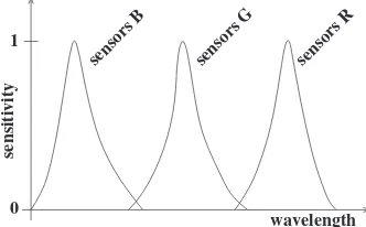
A colour band is a range of wavelengths of the electromagnetic spectrum, over which the sensors we use to capture an image have nonzero sensitivity. Typical colour images consist of three colour bands. This means that they have been captured by three different sets of sensors, each set made to have a different sensitivity function. Figure 1.1 shows typical sensitivity curves of a multispectral camera.
All the methods presented in this book, apart from those in Chapter 7, will refer to single band images.
sensors B sensors G sensors R
wavelength
sensitivity
1
0
Figure 1.1: The spectrum of the light which reaches a sensor is multiplied with the sensitivity function of the sensor and recorded by the sensor. This recorded value is the brightness of the image in the location of the sensor and in the band of the sensor. This figure shows the sensitivity curves of three different sensor types.
Why do most image processing algorithms refer to grey images, while most images we come across are colour images?
For various reasons.
1. A lot of the processes we apply to a grey image can be easily extended to a colour image by applying them to each band separately.
2. A lot of the information conveyed by an image is expressed in its grey form and so colour is not necessary for its extraction. That is the reason black and white television receivers had been perfectly acceptable to the public for many years and black and white photography is still popular with many photographers.
3. For many years colour digital cameras were expensive and not widely available. A lot of image processing techniques were developed around the type of image that was available. These techniques have been well established in image processing.
How is a digital image formed?
Each pixel of an image corresponds to a part of a physical object in the 3D world. This physical object is illuminated by some light which is partly reflected and partly absorbed by it. Part of the reflected light reaches the array of sensors used to image the scene and is responsible for the values recorded by these sensors. One of these sensors makes up a pixel and its field of view corresponds to a small patch in the imaged scene. The recorded value by each sensor depends on its sensitivity curve. When a photon of a certain wavelength reaches the sensor, its energy is multiplied with the value of the sensitivity curve of the sensor at that wavelength and is accumulated. The total energy collected by the sensor (during the exposure time) is eventually used to compute the grey value of the pixel that corresponds to this sensor.
If a sensor corresponds to a patch in the physical world, how come we can have more than one sensor type corresponding to the same patch of the scene?
Indeed, it is not possible to have three different sensors with three different sensitivity curves corresponding exactly to the same patch of the physical world. That is why digital cameras have the three different types of sensor slightly displaced from each other, as shown in figure 1.2, with the sensors that are sensitive to the green wavelengths being twice as many as those sensitive to the blue and the red wavelengths. The recordings of the three sensor types are interpolated and superimposed to create the colour image. Recently, however, cameras have been constructed where the three types of sensor are combined so they exactly exist on top of each other and so they view exactly the same patch in the real world. These cameras produce much sharper colour images than the ordinary cameras.
R G RG
G G
R G
G R R
G R G R G
B B B
B
B B B
B B
G
G G
G G G R
R G G
G
Figure 1.2: TheRGB sensors as they are arranged in a typical digital camera.
What is the physical meaning of the brightness of an image at a pixel position?
Example 1.1
You are given a triple array of3×3sensors, arranged as shown in figure 1.3, with their sampled sensitivity curves given in table 1.1. The last column of this table gives in some arbitrary units the energy,Eλi, carried by photons with wavelength λi.
Wavelength Sensors B Sensors G Sensors R Energy
λ0 0.2 0.0 0.0 1.00
λ1 0.4 0.2 0.1 0.95
λ2 0.8 0.3 0.2 0.90
λ3 1.0 0.4 0.2 0.88
λ4 0.7 0.6 0.3 0.85
λ5 0.2 1.0 0.5 0.81
λ6 0.1 0.8 0.6 0.78
λ7 0.0 0.6 0.8 0.70
λ8 0.0 0.3 1.0 0.60
λ9 0.0 0.0 0.6 0.50
Table 1.1: The sensitivity curves of three types of sensor for wavelengths in the range [λ0, λ9], and the corresponding energy of photons of these particular wavelengths in some arbitrary units.
The shutter of the camera is open long enough for 10 photons to reach the locations of the sensors.
(2,2)
(3,1)
B
B
B
B
B
B
R
R
R
G
G
G
G
R G
B
B
B
(2,1)
(2,3)
(3,2) (3,3)
(1,1) (1,2) (1,3)
G R
R
G
R
G
R
G
R
Figure 1.3: Three 3×3 sensor arrays interlaced. On the right, the loca-tions of the pixels they make up. Although the three types of sensor are slightly misplaced with respect to each other, we assume that each triplet is coincident and forms a single pixel.
The wavelengths of the photons that reach the pixel locations of each triple sensor, as identified in figure 1.3, are:
Location (1,1): λ0,λ9,λ9,λ8,λ7,λ8,λ1,λ0,λ1,λ1 Location (1,2): λ1,λ3,λ3,λ4,λ4,λ5,λ2,λ6,λ4,λ5 Location (1,3): λ6,λ7,λ7,λ0,λ5,λ6,λ6,λ1,λ5,λ9 Location (2,1): λ0,λ1,λ0,λ2,λ1,λ1,λ4,λ3,λ3,λ1 Location (2,2): λ3,λ3,λ4,λ3,λ4,λ4,λ5,λ2,λ9,λ4 Location (2,3): λ7,λ7,λ6,λ7,λ6,λ1,λ5,λ9,λ8,λ7 Location (3,1): λ6,λ6,λ1,λ8,λ7,λ8,λ9,λ9,λ8,λ7 Location (3,2): λ0,λ4,λ3,λ4,λ1,λ5,λ4,λ0,λ2,λ1 Location (3,3): λ3,λ4,λ1,λ0,λ0,λ4,λ2,λ5,λ2,λ4
Calculate the values that each sensor array will record and thus produce the three photon energy bands recorded.
We denote bygX(i, j)the value that will be recorded by sensor typeX at location(i, j). For sensors R,GandB in location(1,1), the recorded values will be:
gR(1,1) = 2Eλ0×0.0 + 2Eλ9×0.6 + 2Eλ8×1.0 + 1Eλ7×0.8 + 3Eλ1×0.1 = 1.0×0.6 + 1.2×1.0 + 0.7×0.8 + 2.85×0.1
= 2.645 (1.2)
gG(1,1) = 2Eλ0×0.0 + 2Eλ9×0.0 + 2Eλ8×0.3 + 1Eλ7×0.6 + 3Eλ1×0.2 = 1.2×0.3 + 0.7×0.6 + 2.85×0.2
= 1.35 (1.3)
gB(1,1) = 2Eλ0×0.2 + 2Eλ9×0.0 + 2Eλ8×0.0 + 1Eλ7×0.0 + 3Eλ1×0.4 = 2.0×0.2 + 2.85×0.4
= 1.54 (1.4)
Working in a similar way, we deduce that the energies recorded by the three sensor arrays are:
ER =
⎛
⎝
2.645 2.670 3.729 1.167 4.053 4.576 4.551 1.716 1.801
⎞
⎠
EG =
⎛
⎝
1.350 4.938 4.522 2.244 4.176 4.108 2.818 2.532 2.612
⎞
⎠
EB =
⎛
⎝
1.540 5.047 1.138 4.995 5.902 0.698 0.536 4.707 5.047
⎞
256×256 pixels 128×128 pixels
64×64 pixels 32×32 pixels
Figure 1.4: Keeping the number of grey levels constant and decreasing the number of pixels with which we digitise the same field of view produces the checkerboard effect.
Why are images often quoted as being 512×512, 256×256, 128×128 etc?
Many calculations with images are simplified when the size of the image is a power of 2. We shall see some examples in Chapter 2.
How many bits do we need to store an image?
The number of bits, b, we need to store an image of sizeN×N, with 2mgrey levels, is:
b=N×N×m (1.6)
What determines the quality of an image?
The quality of an image is a complicated concept, largely subjective and very much application dependent. Basically, an image is of good quality if it is not noisy and
(1) it is not blurred; (2) it has high resolution; (3) it has good contrast.
What makes an image blurred?
Image blurring is caused by incorrect image capturing conditions. For example, out of focus camera, or relative motion of the camera and the imaged object. The amount of image blurring is expressed by the so calledpoint spread functionof the imaging system.
What is meant by image resolution?
The resolution of an image expresses how much detail we can see in it and clearly depends on the number of pixels we use to represent a scene (parameterN in equation (1.6)) and the number of grey levels used to quantise the brightness values (parametermin equation (1.6)). Keeping mconstant and decreasing N results in the checkerboard effect (figure 1.4). KeepingN constant and reducingmresults in false contouring(figure 1.5). Experiments have shown that the more detailed a picture is, the less it improves by keepingN constant and increasingm. So, for a detailed picture, like a picture of crowds (figure 1.6), the number of grey levels we use does not matter much.
Example 1.2
Assume that the range of values recorded by the sensors of example 1.1 is from 0 to 10. From the values of the three bands captured by the three sets of sensors, create digital bands with 3 bits each (m= 3).
For 3-bit images, the pixels take values in the range [0,23
−1], ie in the range [0,7]. Therefore, we have to divide the expected range of values to 8 equal intervals: 10/8 = 1.25. So, we use the following conversion table:
This mapping leads to the following bands of the recorded image.
R=
⎛
⎝
2 2 2 0 3 3 3 1 1
⎞
⎠ G=
⎛
⎝
1 3 3 1 3 3 2 2 2
⎞
⎠ B=
⎛
⎝
1 4 0 3 4 0 0 3 4
⎞
⎠ (1.7)
m= 8 m= 7 m= 6
m= 5 m= 4 m= 3
m= 2 m= 1
Figure 1.5: Keeping the size of the image constant (249×199) and reducing the number of grey levels (= 2m) produces false contouring. To display the images, we always map the
256 grey levels (m= 8) 128 grey levels (m= 7)
64 grey levels (m= 6) 32 grey levels (m= 5)
16 grey levels (m= 4) 8 grey levels (m= 3)
4 grey levels (m= 2) 2 grey levels (m= 1)
What does “good contrast” mean?
Good contrast means that the grey values present in the image range from black to white, making use of the full range of brightness to which the human vision system is sensitive.
Example 1.3
Consider each band created in example 1.2 as a separate grey image. Do these images have good contrast? If not, propose some way by which bands with good contrast could be created from the recorded sensor values.
The images created in example 1.2 do not have good contrast because none of them contains the value 7 (which corresponds to the maximum brightness and which would be displayed as white by an image displaying device).
The reason for this is the way the quantisation was performed: the look up table created to convert the real recorded values to digital values took into consideration the full range of possible values a sensor may record (ie from 0 to 10). To utilise the full range of grey values for each image, we should have considered the minimum and the maximum value of its pixels, and map that range to the8 distinct grey levels. For example, for the image that corresponds to bandR, the values are in the range[1.167,4.576]. If we divide this range in8 equal sub-ranges, we shall have:
All pixels with recorded value in the range[0.536,1.20675) get grey value 0 All pixels with recorded value in the range[1.20675,1.8775) get grey value 1 All pixels with recorded value in the range[1.8775,2.54825) get grey value 2 All pixels with recorded value in the range[2.54825,3.219) get grey value 3 All pixels with recorded value in the range[3.219,3.88975) get grey value 4 All pixels with recorded value in the range[3.88975,4.5605) get grey value 5 All pixels with recorded value in the range[4.5605,5.23125) get grey value 6 All pixels with recorded value in the range[5.23125,5.902] get grey value 7
We must create one such look up table for each band. The grey images we create this way are:
R=
⎛
⎝
3 3 6 0 6 7 7 1 1
⎞
⎠ G=
⎛
⎝
0 7 7 1 6 6 3 2 2
⎞
⎠ B=
⎛
⎝
1 6 0 6 7 0 0 6 6
⎞
⎠ (1.8)
Example 1.4
Repeat example 1.3, now treating the three bands as parts of the same colour image.
find the minimum and maximum value over all three recorded bands, and create a look up table appropriate for all bands. In this case, the range of the recorded values is[0.536,5.902]. The look up table we create by mapping this range to the range[0,7]is
All pixels with recorded value in the range[0.536,1.20675) get grey value 0 All pixels with recorded value in the range[1.20675,1.8775) get grey value 1 All pixels with recorded value in the range[1.8775,2.54825) get grey value 2 All pixels with recorded value in the range[2.54825,3.219) get grey value 3 All pixels with recorded value in the range[3.219,3.88975) get grey value 4 All pixels with recorded value in the range[3.88975,4.5605) get grey value 5 All pixels with recorded value in the range[4.5605,5.23125) get grey value 6 All pixels with recorded value in the range[5.23125,5.902] get grey value 7 The three image bands we create this way are:
R=
⎛
⎝
3 3 4 1 5 6 5 1 1
⎞
⎠ G=
⎛
⎝
1 6 5 2 5 5 3 2 3
⎞
⎠ B=
⎛
⎝
1 6 0 6 7 0 0 6 6
⎞
⎠ (1.9)
Note that each of these bands if displayed as a separate grey image may not display the full range of grey values, but it will have grey values that are consistent with those of the other three bands, and so they can be directly compared. For example, by looking at the three digital bands we can say that pixel(1,1) has the same brightness (within the limits of the digitisation error) in bands G or B. Such a statement was not possible in example 1.3 because the three digital bands were not calibrated.
What is the purpose of image processing?
Image processing has multiple purposes.
• To improve the quality of an image in a subjective way, usually by increasing its contrast. This is calledimage enhancement.
• To use as few bits as possible to represent the image, with minimum deterioration in its quality. This is calledimage compression.
• To improve an image in an objective way, for example by reducing its blurring. This is calledimage restoration.
• To make explicit certain characteristics of the image which can be used to identify the contents of the image. This is calledfeature extraction.
How do we do image processing?
Do we use nonlinear operators in image processing?
Yes. We shall see several examples of them in this book. However, nonlinear operators cannot be collectively characterised. They are usually problem- and application-specific, and they are studied as individual processes used for specific tasks. On the contrary, linear operators can be studied collectively, because they share important common characteristics, irrespective of the task they are expected to perform.
What is a linear operator?
Consider Oto be an operator which takes images into images. If f is an image,O(f) is the result of applyingOtof. Ois linear if
O[af+bg] =aO[f] +bO[g] (1.10)
for all imagesf andgand all scalarsaandb.
How are linear operators defined?
Linear operators are defined in terms of their point spread functions. The point spread function of an operator is what we get out if we apply the operator on a point source:
O[point source] ≡ point spread function (1.11)
Or
O[δ(α−x, β−y)] ≡ h(x, α, y, β) (1.12)
whereδ(α−x, β−y) is a point source of brightness 1 centred at point (x, y).
What is the relationship between the point spread function of an imaging device and that of a linear operator?
They both express the effect of either the imaging device or the operator on a point source. In the real world a star is the nearest to a point source. Assume that we capture the image of a star by using a camera. The star will appear in the image like a blob: the camera received the light of the point source and spread it into a blob. The bigger the blob, the more blurred the image of the star will look. So, the point spread function of the camera measures the amount of blurring present in the images captured by this camera. The camera, therefore, acts like a linear operator which accepts as input the ideal brightness function of the continuous real world and produces the recorded digital image. That is why we use the term “point spread function” to characterise both cameras and linear operators.
How does a linear operator transform an image?
If the operator islinear, when the point source isatimes brighter, the result will beatimes higher:
An image is a collection of point sources (thepixels) each with its own brightness value. For example, assuming that an imagef is 3×3 in size, we may write:
f =
We may say that an image is the sum of these point sources. Then the effect of an operator characterised by point spread functionh(x, α, y, β) on an imagef(x, y) can be written as: Applying an operator on it produces the point spread function of the operator times the strength of the source, ie times the grey valuef(x, y) at that location. Then, as the operator is linear, we sum over all such point sources, ie we sum over all pixels.
What is the meaning of the point spread function?
The point spread functionh(x, α, y, β) expresses how much the input value at position (x, y) influences the output value at position (α, β). If the influence expressed by the point spread function is independent of the actual positions but depends only on therelative position of the influencing and the influenced pixels, we have ashift invariantpoint spread function:
h(x, α, y, β) =h(α−x, β−y) (1.16)
Then equation (1.15) is aconvolution:
g(α, β) =
If the columns are influenced independently from the rows of the image, then the point spread function isseparable:
h(x, α, y, β)≡hc(x, α)hr(y, β) (1.18)
The above expression serves also as the definition of functionshc(x, α) and hr(y, β). Then equation (1.15) may be written as a cascade of two 1D transformations:
g(α, β) =
If the point spread function is both shift invariant and separable, then equation (1.15) may be written as a cascade of two 1D convolutions:
Box 1.1. The formal definition of a point source in the continuous domain
Let us define an extended source of constant brightness
δn(x, y)≡n2
rect(nx, ny) (1.21)
wherenis a positive constant and
rect(nx, ny) ≡
1 inside a rectangle|nx| ≤ 1 2,|ny| ≤
1 2
0 elsewhere (1.22)
The total brightness of this source is given by
+∞
−∞
+∞
−∞
δn(x, y)dxdy = n2 +∞
−∞
+∞
−∞
rect(nx, ny)dxdy
area of rectangle
= 1 (1.23)
and is independent ofn.
Asn→+∞, we create a sequence,δn, of extended square sources which gradually shrink with their brightness remaining constant. At the limit,δn becomes Dirac’s delta function
δ(x, y)
= 0 forx=y= 0
= 0 elsewhere (1.24)
with the property:
+∞
−∞
+∞
−∞
δ(x, y)dxdy = 1 (1.25)
Integral
+∞
−∞
+∞
−∞
δn(x, y)g(x, y)dxdy (1.26)
is the average of imageg(x, y) over a square with sides 1
n centred at (0,0). At the limit,
we have
+∞
−∞
+∞
−∞
δ(x, y)g(x, y)dxdy = g(0,0) (1.27)
which is the value of the image at the origin. Similarly,
+∞
−∞
+∞
−∞
is the average value ofg over a square 1
This equation is called theshifting propertyof the delta function. This equation also shows thatany imageg(a, b) can be expressed as a superposition of point sources.
Example 1.5
The following 3×3 image
f =
h(3,1,3,1) = 0.8 h(3,1,3,2) = 0.5 h(3,1,3,3) = 0.5 h(3,2,3,1) = 0.5
h(3,2,3,2) = 0.5 h(3,2,3,3) = 0.8 h(3,3,3,1) = 0.4 h(3,3,3,2) = 0.4
h(3,3,3,3) = 1.0
Work out the output image.
The point spread function of the operatorh(x, α, y, β)gives the weight with which the pixel value at input position (x, y) contributes to output pixel position (α, β). Let us call the output imageg(α, β). We show next how to calculate g(1,1). For g(1,1), we need to use the values of h(x,1, y,1) to weigh the values of pixels (x, y)of the input image:
g(1,1) =
3
x=1 3
y=1
f(x, y)h(x,1, y,1)
= f(1,1)h(1,1,1,1) +f(1,2)h(1,1,2,1) +f(1,3)h(1,1,3,1) +f(2,1)h(2,1,1,1) +f(2,2)h(2,1,2,1) +f(2,3)h(2,1,3,1) +f(3,1)h(3,1,1,1) +f(3,2)h(3,1,2,1) +f(3,3)h(3,1,3,1) = 2×1.0 + 6×1.0 + 1×0.8 + 4×0.8 + 7×0.5 + 3×0.9
+5×0.7 + 7×0.8 = 27.3 (1.32)
Forg(1,2), we need to use the values ofh(x,1, y,2):
g(1,2) =
3
x=1 3
y=1
f(x, y)h(x,1, y,2) = 20.1 (1.33)
The other values are computed in a similar way. Finally, the output image is:
g=
⎛
⎝
27.3 20.1 18.9 19.4 16.0 18.4 16.0 29.3 33.4
⎞
⎠ (1.34)
Example 1.6
Is the operator of example 1.5 shift invariant?
No, it is not. For example, pixel (2,2)influences the value of pixel (1,2)with weight