www.elsevier.com / locate / econbase
A new definition for time-dependent price mean reversion in
commodity markets
a b ,
*
cAhmet E. Kocagil , Norman R. Swanson
, Tian Zeng
a
Pennsylvania State University, University Park, PA, USA
b
Department of Economics, Texas A&M University, Academic Building West, College Station, TX 77843-4228, USA
c
Aeltus Investment Management, Inc., Hartford, CT, USA
Received 9 February 2000; accepted 20 September 2000
Abstract
In this note we propose a time-dependent definition of mean reversion, and empirically compare our definition with two former definitions. We show that the incidence of mean reversion is approximately 30–40% less under the new and more robust definition. 2001 Elsevier Science B.V. All rights reserved.
Keywords: Mean reversion; Anticipated spot prices; Forecastability; Futures prices; Term structure; Hedging; Interest rate
shocks; Convenience yield shocks
JEL classification: C20; G12; G14
1. Introduction
The theoretical significance of price mean reversion in financial markets has long been recognized
1
as crucial in discussions of predictive ability, arbitrage, hedging behavior, and derivative valuation. One feature of empirical investigations to date which attempt to verify the presence of mean reversion is that they all focus on static examinations of financial variables. In this note we recognize the potential significance of time variation in price reversion, and propose a time-dependent definition of mean reversion, which is based on the term-structure of prices. We empirically compare our definition with two other related definitions, and show that when mean reversion is allowed to be sample
*Corresponding author. Tel.: 11-979-845-7351; fax:11-979-847-8757.
E-mail address: [email protected] (N.R. Swanson).
1
See Miller et al. (1994), Park (1996), Poterba and Summers (1988), and the references contained therein for further related discussion.
2
dependent, the incidence of mean reversion is approximately 30–40% less when our definition is used. We discuss reasons for this as well as pointing out a number of advantages of our definition.
2. Defining mean reversion
According to the theory of storage, futures prices with a delivery date of t1m at time t, say F (m),
t
where P is the spot price, r (m) is the interest rate over the remaining life of the futures contract, andt t
c (m) is the convenience yield net of storage costs. The spread between the interest rate and thet
convenience yield, S 5r 2c , can be thought as the slope of the term structure of futures prices. We
t t t
take Eq. (1) as given in the sequel.
Many authors have investigated mean reversion in prices and returns, including Bollerslev and Mikkelsen (1996), Fama and French (1988a,b), and Park (1996). Bessembinder et al. (1995), for example, examine the presence of mean reversion in the above framework, where spot and future equilibrium prices are simultaneously determined in the absence of any arbitrage opportunities, and assuming that there is negative correlation between the futures risk premium and spot prices. This implies that anticipated mean reversion in spot prices is associated with a concave term structure, i.e. appreciation in intertemporal futures prices decelerates when spot prices rise. Accordingly, denoting the elasticity of futures price with respect to spot prices as ´ , mean reversion is said to occur
E(P )P,t
when ´ ,1, i.e.
E(P )P,t
3
Definition 1. There is mean reversion if dS / dP is negative (or ´ ,1).
t t FP,t
This definition is appealing in a static context, and is consistent with the Samuelson (1965)
2
By sample dependence, we mean that alternative windows of historical data available at different calendar dates are used to assess whether there is mean reversion at any given point in time.
3
This follows by first defining p(m)5ln[E (P ) /F (m)], where p(m) is the bias in the futures spot price prediction
t t t1m t t
when that price is predicted using F (m). Then, it follows that the current price can be written ast
proposition that futures prices vary less than spot prices. It also implies that temporary components of price shocks will be dampened over time when there is mean reversion. As Fama and French (1988a,b) suggest, offsetting effects of demand and supply on future spot prices will be stronger for longer horizons. Correspondingly, expected spot (or futures) price fluctuations reflect mainly
permanent shocks, whereas spot prices are affected by both permanent as well as temporary shocks.
Therefore, it could be argued that, in the absence of other consecutive shocks, spot prices would follow futures prices over time. Accordingly, we might also define mean reversion as:
Definition 2. In the presence of both temporary and permanent shocks, mean reversion in spot prices
occurs if either: (i) P .F and dP ,0, or (ii) P,F and dP .0.
t t t t t t
Assuming nonstationarity of prices, Definition 2 implies that P is not reverting to a stationaryt variable, but to a nonstationary one, F . Accordingly, the spot and futures series should bet
4
cointegrated. In addition, parts (i) and (ii) of Definition 2 are both intuitively appealing as they involve assessing whether spot price changes follow changes in futures markets.
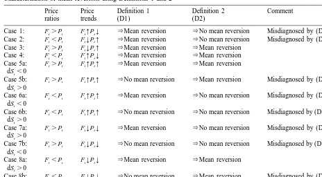
Before proposing our definition of mean reversion, we first outline the predictions of Definitions 1 and 2 under all current spot and futures price combination scenarios. In particular, Table 1 summarizes all of the possible price combinations and displays the implications of using Definitions 1 or 2 to define mean reversion. A comment on the organization of the table will be useful before summarizing the results. That is, note that the sign of dS is not given for Cases 1–4. This is becauset dS must be greater than zero for Cases 1 and 3 and less than zero for Cases 2 and 4. This in turnt follows directly from Eq. (1), and from the price ratios and price trends given in columns 2 and 3 in the table. On the other hand, dS can be both positive and negative whenever both spot and futurest prices are increasing or decreasing (Cases 5–8). Thus, we have partitioned these cases into parts a and b, depending on whether prices are increasing or decreasing. To illustrate, note that in Case 4, dS .0
t and P is decreasing, so that dS / dP is negative, implying mean reversion according to Definition 1.t t t In addition, mean reversion is clearly implied by Definition 2 in this case. Thus, both definitions correctly find mean reversion when prices are evolving according to Case 4, given that spot and futures prices are clearly converging over time.
However, overall examination of the entries in Table 1 reveals that despite its intuitive appeal, Definition 1 exhibits some shortcomings when used to define mean reversion. For instance, note that in Cases 1 and 2, ´ ,1. Thus, Definition 1 suggests that mean-reverting behavior is present in
FP,t
these cases, which is clearly a counterintuitive outcome, as noted in the final column of the table. Likewise, Cases 6a and 7a also correspond to mean-reverting behavior according to Definition 1, even though F and P are moving apart from each other in these cases. For example, in Case 6a, wheret t dS ,0, which implies that P is growing faster than F , note that F is initially lower than P (see
t t t t t
4
Table 1
Characterization of mean reversion using Definitions 1 and 2
Price Price Definition 1 Definition 2 Comment
ratios trends (D1) (D2)
column 2). Since both prices are increasing over time (see column 3), this in turn suggests that spot prices are increasing faster than futures prices, and as futures prices are initially lower, spot and futures prices must be moving apart, or diverging, over time — so that mean reversion in this case is counterintuitive.
It should perhaps be stressed that these counterintuitive findings arise because we are evaluating our baseline definition (Definition 1) in a dynamic setting rather than in the static setting. Notice also that Definition 2 erroneously finds mean reversion in Cases 5b and 8b, although Definition 1 does not. Noting the obvious complementarity between the two definitions, it should not come as a surprise that virtually all misdiagnosed cases (with the exception of Cases 6b and 7b) can be avoided by defining mean reversion as the intersection of Definitions 1 and 2. In particular, consider:
Definition 3. There exists mean reversion among anticipated spot price returns if
1. ´ ,1, and
FP,t
2. either: (i) P .F and dP ,0, or (ii) P ,F and dP .0.
t t t t t t
Proposition 4. Assume that Eq. (1) holds, and S and P are twice continuously differentiable witht t
5
respect to P . Then the following relationships exist between Definitions 1 and 2:t
(i ) Mean reversion (Definition 1)⇔dS /dP ,0, and
t t
(ii ) Mean reversion (Definition 2)⇔(dS /dP )(dS /S ).0.
t t t t
Part (i) of Proposition 4 states that the term structure becomes flatter as spot prices increase. In order to satisfy Definition 2 in this case, S must be negative. However, note that Definition 2 also holdst when the term structure becomes steeper, as long as the rate of growth of the basis is positive, and spot prices follow futures prices. In addition, note that under the same conditions as those stated in Proposition 4, the intersection between Definitions 1 and 2, i.e. Definition 3, implies that dS /S ,0.
t t Thus, Definition 3 holds when the market is in contango (S .0) or in backwardation (S ,0), as
t t
long as the basis is shrinking. In other words, it implies that, for mean reversion to exist, the absolute value of the basis should be shrinking over time, which is a condition that is consistent with the fundamentals of the theory of futures markets.
3. Empirical results and conclusions
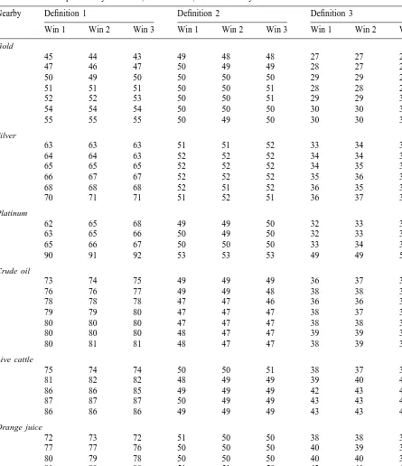
We calculate frequencies of mean reversion by examining daily spot and futures prices for four mineral (crude oil, gold, silver and platinum), two agricultural (orange juice and live cattle), and two financial (treasury bonds and S&P500) markets. In particular, we determine whether mean reversion exists using window sizes of 60, 120, and 240 days for each day between 4 / 1 / 82 and 10 / 31 / 95. Entries reported in Table 2 correspond to the percentage of times mean reversion is found according to Definitions 1–3 at the end of each day in the sample period. All data were obtained from the CRB
6
Commodity database.
A number of clear results emerge upon inspection of the percentages given in Table 2. First, differences in window size do not have an appreciable impact on the incidence of mean reversion,
5
For the proof of Part (i), see Footnote 3. Part (ii) of Proposition 4 can be proven by noting that Part (2) of Definition 3 can be stated equivalently as (F2P )dP.0. However, from the definition of S it follows that the sign of S dP is the same
t t t t t t
which is clearly positive as long as S dP.0. As S dP.0 is implied by Definition 2, the if part of the proposition follows.
t t t t
The only if part of the proof follows by writing the RHS of Part (ii) as 2
Table 2
a Mean reversion frequencies by definition, data window, and commodity
Nearby Definition 1 Definition 2 Definition 3
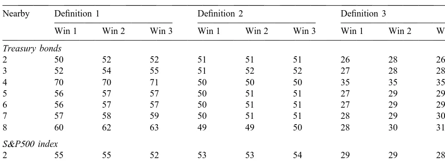
Table 2. Continued
Nearby Definition 1 Definition 2 Definition 3
Win 1 Win 2 Win 3 Win 1 Win 2 Win 3 Win 1 Win 2 Win 3
Treasury bonds
2 50 52 52 51 51 51 26 28 26
3 52 54 55 51 52 52 27 28 28
4 70 70 71 50 50 50 35 35 35
5 56 57 57 50 51 51 27 29 29
6 56 57 57 50 51 51 27 29 29
7 57 58 59 50 51 51 28 29 30
8 60 62 63 49 49 50 28 30 31
S&P500 index
2 55 55 52 53 53 54 29 29 28
3 56 55 54 53 53 53 30 30 29
a
Frequencies are calculated by counting the incidence of daily mean reversion between 4 / 1 / 82 and 10 / 31 / 95. The number of trading days used for each successive daily calculation was fixed at 60 (Win 1), 120 (Win 2), or 240 days (Win 3). All figures can be interpreted as percentages, e.g. 505mean reversion for 50% of the days examined.
suggesting that our findings are robust to the length of the sample period used. Second, Definition 1 implies that mean reversion holds 90% of the time in some cases, with most figures falling in the 60–80% range. However, mean reversion percentages are somewhat lower based on Definition 2, and substantially lower for Definition 3, which is consistent with our observation that Definition 1 misdiagnoses some market situations as being ‘mean-reverting’. In particular, percentages based on Definition 2 are concentrated around 50%, regardless of commodity and nearby contract. This finding suggests that temporary shocks account for as much as 50% of spot price changes. In addition, Definition 3 finds mean reversion only around 30–40% of the time. Finally, it is worth noting that percentages clearly vary the least across nearby contract and across commodity when Definition 3 is used. Thus, we conclude that Definition 3 is not only more intuitively appealing than Definitions 1 and 2, but it also leads to a more robust and substantially reduced estimate of the incidence of mean reversion.
Acknowledgements
The authors are grateful to Eric Ghysels and Frank Hatheway for providing useful comments on an earlier draft of this paper. Swanson would also like to thank the Private Enterprise Research Center and the Bush Program in the Economics of Public Policy for research support. Parts of this paper were written while the second author was visiting the University of California, San Diego.
References
Bollerslev, T., Mikkelsen, H.O., 1996. Modeling and pricing long memory in stock market volatility. Journal of Econometrics 73, 151–184.
Christoffersen, P., Diebold, F.X., 1997. Cointegration and long-horizon forecasting. Journal of Business and Economic Statistics, forthcoming.
Engle, R.F., Granger, C.W.J., 1987. Co-integration and error correction: representation, estimation, and testing. Econometrica 55, 251–276.
Fama, E.F., French, K.R., 1988a. Business cycles and the behavior of metals prices. Journal of Finance 43, 1075–1093. Fama, E.F., French, K.R., 1988b. Permanent and temporary components of stock prices. Journal of Political Economy 96,
246–273.
Chernov, M., Ghysels, E., 1999. A study towards a unified approach to the joint estimation of objective and risk neutral measures for the purpose of options valuation. Journal of Financial Economics, forthcoming.
Johansen, S., 1988. Statistical analysis of cointegration vectors. Journal of Economics and Dynamics Control 12, 231–254. Johansen, S., 1991. Estimation and hypothesis testing of cointegration vectors in Gaussian vector autoregressive models.
Econometrica 59, 1551–1580.
Miller, M.H., Muthuswamy, J., Whaley, R.E., 1994. Mean reversion of Standard & Poor’s 500 index based changes: arbitrage-induced or statistical illusion. Journal of Finance 49, 479–513.
Park, T.H., 1996. Mean reversion of interest-rate term premiums and profits from trading strategies with treasury futures spreads. Journal of Futures Markets 16, 331–352.
Poterba, J., Summers, L., 1988. Mean reversion in stock prices: evidence and implications. Journal of Financial Economics 22, 27–59.