www.elsevier.com / locate / econbase
Measurement error in a single regressor
*
Erik Meijer , Tom Wansbeek
Department of Econometrics, University of Groningen, P.O. Box 800, 9700 AV Groningen, The Netherlands
Received 20 December 1999; accepted 15 June 2000
Abstract
For the setting of multiple regression with measurement error in a single regressor, we present some very simple formulas to assess the result that one may expect when correcting for measurement error. It is shown where the corrected estimated regression coefficients and the error variance may lie, and how the t-value behaves. 2000 Elsevier Science S.A. All rights reserved.
Keywords: Attenuation; t-statistic; CALS
JEL classification: C21; C52
1. Introduction
In the applied econometrics literature of the cross-sectional type, one often meets the case of a regression equation being estimated where the regressor set includes a number of control variables to account for population heterogeneity in addition to one regressor focal to the topic under study. This variable is often theory-based and is not directly observable, for conceptual or practical reasons. Examples are, among many others, consumption models relating consumption to permanent income, labor supply models relating hours to wage per hour, models assessing the policy impact of central bank independence, and investment models relating investment to Tobin’s q. The case of multiple regression with measurement error in a single but interesting regressor may hence be considered almost generic. It is generally appreciated that in such cases OLS gives an inconsistent result. Most textbooks discuss this and come up with solutions. For example, when the measurement error variance is known, the OLS results can be adapted to construct a consistent estimator. However, the approach most frequently mentioned is the use of instrumental variables. Instruments can sometimes be found by further scrutinizing the available data set but they can also be constructed from the data already
*Corresponding author. Tel.: 131-50-363-3793; fax:131-50-363-3720. E-mail address: [email protected] (E. Meijer).
employed for estimating the model. For example, when the variables are non-normal, the model y5xb1u, with x subject to measurement error, can be consistently estimated with x*y as instrument, as was shown by Lewbel (1997), who elaborated on this simple idea to suggest a wide set of IV’s. Be it as it is, before entering on such a course it may be worthwhile to know what to expect when applying methods that correct for measurement error in a single regressor in a multiple-regression setting; see e.g. Wansbeek and Meijer (in press) for an overview. To that end we group, in this note, a number of partly new results that are very simple to apply and that are intended to provide guidance to the applied researcher. These results build on the output of OLS estimation of the model and show how the results change when different values of the measurement error variance (f) are considered. The set-up is as follows. After summarizing, in Section 2, the basic results for regression with measurement error in multiple regression, we narrow the results down for the case of measurement error in a single variable in Section 3. It is shown where the estimate of the regression coefficients and of the residual error variance may lie depending on f. The situation is depicted graphically in Section 4. A consistent estimator of the asymptotic variance is given in Section 5. As stated above, the mismeasured variable is often the core variable in the research, and that makes an investigation of the correction procedure for its coefficient estimate especially interesting. As Section 6 shows, increasing values of f correspond with increasing values of the estimate of its asymptotic variance. This increase outpaces the increase in coefficient estimate and the t-value is monotonously decreasing. The relationship between the measurement error variance and the t-value is given explicitly below. This relationship can be of direct use in applied work, where t-values are assigned a dominant role, since the impact of f on the t-value can be assessed directly. In particular, it can be seen at what level of noise in a variable it ‘disappears into insignificance’.
2. Properties of the measurement error model
The standard linear multiple regression model can be written as
y5Jb1´, (1)
where y is an observable N-vector and´ an unobservable N-vector of random variables, assumed i.i.d.
2
with zero expectation and variance s´. The g-vector b is fixed but unknown. The N3g-matrix J
contains the regressors, assumed independent of ´.
If there are errors of measurement in the explanatory variable, J is not observable. Instead, we observe the matrix X5J1V, where V (N3g) is a matrix of measurement errors. Its rows are assumed to be i.i.d. with zero expectation and covariance matrix V ( g3g) and uncorrelated with J
and ´.
Define the sample second-moment matrices of J and X:
1 1
] ]
KN;NJ9J; AN;NX9X. Note that AN is observable but K is not.N
elements as unknown fixed parameters. Under the latter interpretation, the elements ofJ are supposed to be random variables. The assumption p lim KN5K, with K a positive definite g3g-matrix, is meant to cover both cases. As a consequence, A;p lim AN5K1V.
21 2 21 2
Let b;(X9X ) X9y and s´;1 /N y9(IN2X(X9X ) X9)y be the usual estimators of b and s´, neglecting measurement error. As is well-known, these estimators are inconsistent:
21
p lim b5A (A2V)b
2 2
p lim s´5s´1b9V( p lim b).
If V is known, Slutsky’s theorem implies that
21
are consistent. The asymptotic distribution of these consistent estimators for both the functional and the structural model is given by
21 21
3. Measurement error in a single regressor
We now consider the case where there is measurement error in a single regressor only. Without loss of generality we take this to be the first regressor. Then
9
V5fe e ,1 1 (5)
with e the first unit vector, and1 f the variance of the measurement error in the first regressor. To elaborate this case, the following notation is used:
21
values of f deemed relevant such thatu .0; this holds anyhow in the limit. Substitution of (5) in (2) using (6c) gives
21
ˆ
9
9
b5(AN2fe e )1 1 A bN 5(Ig1ufae )b1
5b1(ufb )a1 5b1la, (7)
with b the first element of b and1
l;ufb .1 (8)
ˆ ˆ
In particular, the first element b1 of b can be written as
ˆ
b15(11ufa)b15ub .1 (9)
ˆ
We assume b1.0 without loss of generality, hence b1$0. So (9) gives the correction for the downward bias when estimating b1 by OLS if there is measurement error, and (7) shows, for all elements ofb jointly, that this correction is along a line inb-space, from b in the direction given by the first column of the inverse of X9X.
2
We now consider the estimation of s´. Combining (3), (5), (8), and (9) gives
2 2 ˆ 2 ˆ
as a consistent estimator given a value for f.
Restricting this estimator to nonnegative values imposes an upper limit on the values off that one may wish to consider. Putting (10) to zero and solving gives
1
a 2
ˆ ]
b1 max5umaxb15b11b s´
1
as the upper bound on the estimator of b1.
4. A graphical illustration
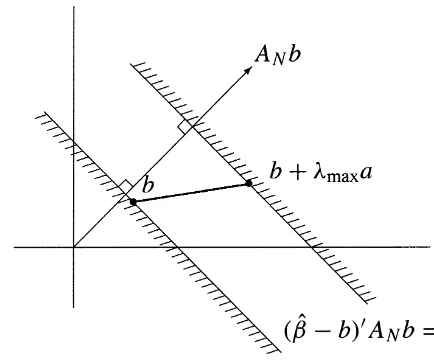
Adapting from Bekker et al. (1984) we can illustrate the above graphically. Let us first consider the case of generalV$0, and assume that the values considered forV satisfyV,A . (Again, this holdsN anyhow in the limit.) Hence
21 21
(AN2V) 2AN $0, (13)
with equality holding only if V50. An implication of (2) is
21
with equality holding only if b50. So, whatever V may be, the corrected estimators lie in b-space ˆ
beyond the plane (b2b)9A bN 50, as seen from the origin. This is the plane through b perpendicular to A b.N
2
ˆ
We now consider the implication of s´$0 or
2
So the measurement-error corrected estimator cannot lie beyond the plane (b2b)9A bN 5s . This´
ˆ
plane is parallel to the plane (b2b)9A bN 50, further away from the origin. The situation is
ˆ
9
illustrated in Fig. 1. The set of b’s compatible withV5fe e is given by the line segment between1 1
the two planes, ranging from b to b1lmaxa.
5. Estimating the asymptotic variance
ForV as in (5) with givenf, we can derive the asymptotic variance of the estimators (9) and (10) by elaborating (4) for this special case. More interestingly, we elaborate consistent estimation of this
2
ˆ
variance for b based on the consistent estimators forb ands´. We consider the various terms in (4) in turn.
2 2 2
ˆ Fig. 1. Admissible values ofb.
2 ˆ2 2 2 2 2
ˆ
s´1fb1 5s´2lb11u fb15s´2lb11ulb1
2 2 2 2
5s´1(u21)lb15s´1ufalb15s´1l a.
21
9
219
Next, using (6d) and (9), v5K Vb5f(A2fe e )1 1 e e1 1b is consistently estimated by
21 ˆ ˆ 2
9
9
f(AN2fe e )1 1 e e1 1b5ufb1a5u fb a1 5ula,
21 21
9
9
and, using (6a)—(6c), K AK 5(A2fe e )A(A1 1 2fe e ) is estimated by1 1
21 21 21
9
9
9
9
(AN2fe e )1 1 A (AN N2fe e )1 1 5(Ig1ufae )A1 N (Ig1ufae )1
21
5AN 1uf(u11)aa9. ˆ
Putting these results together gives for b:
2
2 2 21 2 2
ˆ
(asy.var.b)5(s´1l a)(AN 1uf(u11)aa9)1u l aa9, (16)
2 21
which of course reduces to s A´ N when there is no measurement error.
6. The t-value for the first regression coefficient
For the estimator of the coefficient of the first regressor, taking the upper-left element in (16) gives
2
2 2 2 2 2 2
ˆ
(asy.var.b1) 5(s´1l a)(a1uf(u 11)a )1u l a 2 2 2
5u a(s´12l a).
]
The t-statistic corresponding with a measurement error of size f is, using (9) and (17), given by
]
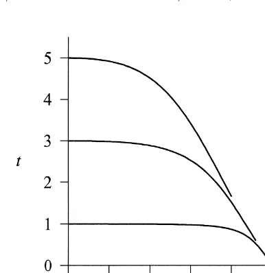
with hf;lat /b0 15(u21)t . After some straightforward calculations there appears to hold0
illustrates the behavior of t , forf a51 and N5100, for various values of t . Substitution of (17) in0
Sometimes it is of interest to see which level off corresponds with a given t-value. Let this value be t . This corresponds with* f5f* satisfying
In particular, one may be interested to see, by putting t at the conventional level of 2, what level of*
noise in a variable makes its estimated coefficient disappear into insignificance.
Acknowledgements
We thank Paul Bekker and Ton Steerneman for their valuable comments.
References
Bekker, P.A., Kapteyn, A., Wansbeek, T.J., 1984. Measurement error and endogeneity in regression: Bounds for ML and 2SLS estimates. In: Dijkstra, T.K. (Ed.), Misspecification Analysis. Springer, Berlin, pp. 85–103.
Kapteyn, A., Wansbeek, T.J., 1984. Errors in variables: Consistent Adjusted Least Squares (CALS) estimation. Communica-tions in Statistics, Theory and Methods 13, 1811–1837.
Lewbel, A., 1997. Constructing instruments for regressions with measurement error when no additional data are available, with an application to patents and R&D. Econometrica 65, 1201–1213.