www.elsevier.nl / locate / econbase
Understanding pooled subjective probability estimates
a ,* b
Thomas S. Wallsten , Adele Diederich
a
Department of Psychology, University of North Carolina, Chapel Hill, NC 27599-3270, USA b
¨
Universitat Oldenburg, Oldenburg, Germany
Received 4 August 1998; received in revised form 19 January 2000; accepted 25 January 2000
Abstract
Decision makers often must pool probability estimates from multiple experts before making a choice. Such pooling sometimes improves accuracy and other times diagnosticity. This article uses a cognitive model of the judge and the decision maker’s classification of the information to explain why. Given a very weak model of the judge, the important factor is the degree to which their information bases are independent. The article also relates this work to other models in the literature. 2001 Elsevier Science B.V. All rights reserved.
Keywords: Subjective probability; Pooling estimates; Calibration; Diagnosticity
JEL classification: D89
1. Introduction
Decision makers (DMs) often must pool judgments from multiple forecasts before making a choice. Consider the following examples: two medical specialists provide different estimates to an individual regarding the probability that a painful procedure will cure her ailment. Members of a panel of engineers give a product manager an assortment of probability estimates that a particular part will fail under stress. Various intelligence analysts give an army commander conflicting estimates regarding the probability of enemy attack. And, finally, when recommending an air quality standard, a government official must consider probability estimates from multiple experts that at least a given fraction of the population will suffer a particular health effect at a given dose of a pollutant.
*Corresponding author. Tel.:11-919-962-2538; fax:11-919-962-2537. E-mail address: [email protected] (T.S. Wallsten).
In cases such as these, DMs must combine the subjective judgments of other 1
forecasters, presumably but not necessarily experts, prior to taking action. There is a vast literature on rational models for reconciling subjective probability estimates, as well as on the empirical consequences of different combination methods. Clemen (1989), Genest and Zidek (1986), and Wallsten et al. (1997) all provide reviews, while Cooke (1991) devotes a major share of his book to the topic.
To fix intuitions, assume that you have individual probability estimates for a large number of events. Consider two different calibration curves (i.e., graphs of the proportion of the true or correct forecasts as a function of the probability estimates). One is for the typical expert and the other is based on the mean of the experts’ estimates for each event. What relationship would you expect between the two calibration curves? And what factors, if any, would you expect to influence the relationship?
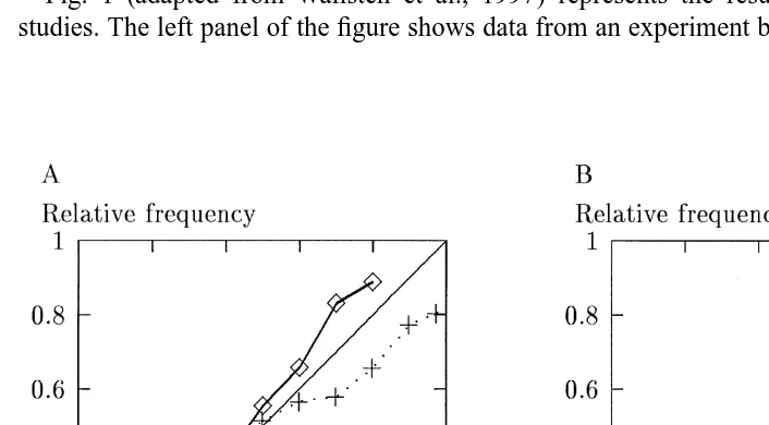
Fig. 1 (adapted from Wallsten et al., 1997) represents the results of two different studies. The left panel of the figure shows data from an experiment by Erev and Wallsten
Fig. 1. Relative frequency as a function of subjective probability category. Data of the left panel are from Erev and Wallsten (1993) for individual subjects (J51) and for probability estimates averaged for each event over all subjects (J560). Data of the right panel are from Wallsten et al. (1993) for individual subjects (J51) and for probability estimates averaged for each statement over all subjects (J521). (Adapted from Wallsten et al., 1997.)
1
(1993). Subjects observed computer displays from which they could infer relative frequency information about 36 distinct events (which among them had 26 different objective probabilities), and provided subjective probability estimates of those events. The right panel of the figure shows results from an experiment by Wallsten et al. (1993), where subjects gave numerical probability estimates that general knowledge statements were true.
The abscissa of each panel is divided into 11 categories centered at 0.025, 0.10, 0.20, . . . ,0.90, 0.975 containing the subjects’ probability estimates. The ordinate of each panel shows the relative frequencies of the events conditional on the estimates. The J51 curves show the average of the calibration curve for individual subjects. They are similar for both studies and show typical results for overconfident judges. The J±1 curves are based on the mean estimates per event (panel A, J560) or per statement (panel B, J521). However, these calibration curves differ considerably. In panel A the relative frequencies for the mean estimates are much closer to the diagonal than are those based on individual estimates. Moreover, the overconfident judgments of in-dividuals have changed to slightly underconfident group judgments. In panel B the relative frequencies for the mean estimates move away from the diagonal; the overconfident individual estimates here combine to form very underconfident, but diagnostic group judgments. Table 1 summarizes these results in the form of the
]
decomposed Brier mean probability score, PS, where CI and DI refer to the calibration
]
2
index and discrimination index, respectively. In both cases, PS is improved (decreased) by averaging the estimates, but the contributions of CI and DI to this decrease are very different.
The purpose of this article is to explain results such as these by simultaneously considering two factors: (1) a cognitive model of the individual judge and (2) information conditions for the DM. The outline of the article is as follows. First we present a very general cognitive model of how the individual judge forms and
Table1
Summary statistics for averaging multiple judgments in two studies
]
Panel Number PS CI DI
judges
1 0.232 0.016 0.181
A 60 0.212 0.006 0.208
1 0.213 0.010 0.181
B 21 0.153 0.024 0.342
]
2 ¯ ¯ ¯
communicates his or her estimates. Then we consider the kind of information on which the DM thinks the judges based their opinions. Next we present a mathematical framework to tie the cognitive and information components together. Then we use our approach to explain the results presented in the Introduction and discuss its further implications. Finally, we relate our model to current approaches to combining prob-abilities.
2. A cognitive model
We begin by considering properties of the experts’ judgments. Our basic assumption is that each expert’s probability estimate depends on two covert components: confidence
3
and random variation. Individuals’ covert confidence depends on what they know and how they think about the events or statements in question. Cognitive theories differ on the nature of this thinking, but all agree that it results in a degree of confidence that we can represent as a latent variable. Random variation represents momentary fluctuations in the sequence of processes that begins with facing the question and ends with giving
4 an estimate.
The covert confidence, X, perturbed by random variation, E, is transformed into an overt estimate, R, such that, for expert or judge j,
Rj5h (X ,E ).j j j (1)
R is a random variable in (0,1); X is either a continuous random variable taking on realj j
values or a discrete random variable in (0,1), depending on the specific assumptions that we make; and E is a continuous random variable taking on real values. h is a functionj j
increasing in both its arguments, which represents judge j’s mapping of randomly perturbed covert confidence into a response. The equation, a generalization of the model in Erev et al. (1994), represents an extremely weak model of the judge, in that it makes no commitment other than the monotonicity of h as to how judges form their covert opinions or translate them into responses.
3
It is common in psychology to distinguish between an individual’s covert processing of information and the resulting overt response. For example, most research on detecting weak signals in noise assumes that an individual’s overt decision depends on an underlying perception relative to an internal response criterion (Green and Swets, 1966). Much judgment research distinguishes how individuals combine the multiple dimensions of a stimulus into covert opinions from how they map the results via a response function into overt expressions (e.g., Birnbaum, 1978).
4
It is immaterial for our purposes whether random variation arises while the judge is considering the available information and arriving at a degree of confidence or while he or she is converting that confidence into an overt expression. In many models of judgment, including the present one, the mathematical consequences are
´
3. Information conditions
The effect of averaging R over J judges depends on the inter-judge relationshipsj
among the X . These relationships may be estimable post hoc. However, a priori the DMj
must make assumptions about them. And appropriate assumptions for a given situation depend on the DM’s view of the judges’ information base, which, in turn, depends on
5
his or her model of the event space. Two different information conditions can be distinguished:
1. The experts share the same source of information, e.g., when estimating a relative frequency, p , based on samples from a population. Generally, this situation occursi
when events can be grouped into classes (or, at least the DM believes that to be the ˆ
case), such that long-run relative frequency estimates of the events, p , are constant ini
(i ) class i. We assume here that all judges have the same opinion, i.e., that Xj5x for event i and all j. (Judges may receive different samples from the information source, but recall from footnote 3 that our model allows us to absorb variability in arriving at a degree of confidence in the error term, E .)j
2. The experts do not share the same source of information (or at least the DM believes that), e.g., when estimating the probability of a particular unique event such as the outcome of an election, based on distinct considerations. Here we assume that judges have different covert opinions, or more generally that the X are not identicallyj
distributed. Now there is a range of cases, depending on the degree to which the judges’ covert opinions are conditionally dependent. At the one, probably rare, extreme the X are conditionally independent, and at the other, probably common,j
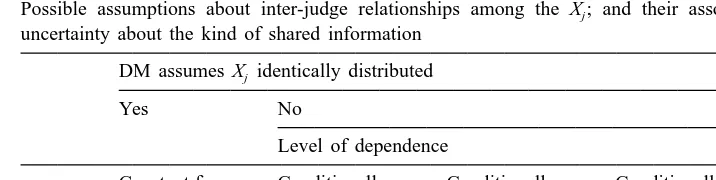
extreme they are conditionally interdependent. Between the two endpoints are several levels of conditional dependence, of which we identify only conditional pairwise independence. Table 2 summarizes the classification of possible inter-judge relation-ships among the X and suggests their association with the DM’s uncertainty aboutj
the kind of shared information.
As we will see in the next section it is a simple matter to derive essentially without additional assumptions the consequences of averaging multiple probability estimates or, more generally, of averaging monotonic increasing transformations of such estimates for Case 1. Under suitable assumptions, one can expect averaging to improve the calibration index, CI.
It is necessary, however, to add a few additional constraints to our model of the judge in order to make progress with the remaining cases in Table 2. Very weak ones suffice for Cases 2 and 3 when we assume that judges partition their covert confidence into a finite number of discrete categories. In this case, X can be taken to represent thej
5
Table 2
Possible assumptions about inter-judge relationships among the X ; and their association with the DM’sj uncertainty about the kind of shared information
DM assumes X identically distributedj
Yes No
Level of dependence
Constant for Conditionally Conditionally Conditionally event i independent pairwise dependent
independent
Case 1 2 3 4
proportion of events judge j assigns to the categories that are true. With a few assumptions, one can expect averaging to improve the discrimination index, DI. Case 4 is the most interesting and realistic case and awaits further work. Next, we present our results for Case 1 and then for Cases 2 and 3.
4. A mathematical framework
Throughout the following we consider the overt estimate and covert confidence of judge j with respect to one particular event, say i. However, it becomes rather messy to
(i ) (i )
include the event in the notation, e.g., Eq. (1) becomes Rj 5h (X ,E ). As noj j j
confusion will arise, we omit explicitly referencing the event. Further, to allow the DM to transform response scales, we introduce a function f that may convert the overt responses, for example, from probability into log-odds. f may be any continuous strictly increasing finitely bounded function.
4.1. Case 1
Our result in this case suggests that averaging multiple estimates (or their transforma-tions) will improve their accuracy (depending on the response function, h ).j
Define
• ERJ;(1 /J )ojE( f(R )), jj 51, . . . ,J, as the average expected (transformed) response of J judges to event i;
• MJ;(1 /J )ojf(h (x ,e )), jj j j 51, . . . ,J (with ej[E ), as the observed mean (trans-j
formed) response of J judges to event i.
For the model presented in Eq. (1) consider the following assumptions:
` 2
Theorem 1. (Case 1) If A1– A3 hold and if oj51Var[ f(R )] /jj , ` then as J→`
MJ→ER a.s.J
Proof. Since the x are constant and E are independent, Rj j5h (x,E ) are independent,j j
j51, . . . ,J. The proof is completed by Kolmogorov’s strong law of large numbers. 4.2. Cases 2 and 3
Although Theorem 1 applies to Cases 2 and 3 as well, it is not useful because in these cases events are unique and therefore only either true or false. For convenience the states of the event are denoted as Si51 and Si50, for true and false events, respectively. As will be shown, with suitable assumptions, averaging leads to highly diagnostic estimates.
Let:
• l, l50,1, . . . ,N , index the Nj j11 underlying probability categories used by judge j, with N being even;j
• X be a discrete random variable taking on values xj jl in (0,1), representing the proportion of events judge j assigns to category l that are true. Without loss of generality let 0,xj 0,xj 1, ? ? ? ,xj,Nj,1.
The claim that covert confidence is categorical with an odd number of categories is descriptively compelling, but we could structure the proof without it. The descriptive merit of defining X in such a way arises from the fact that most judges providej
probability estimates in multiples of 0.1 or 0.05 (see, for example, Wallsten et al., 1993). However, we include the claim not because of its cognitive content, but as a mathematical convenience that simplifies the statements of A4 and A5 below and to some degree the proof. Moreover, the claim itself is not very restrictive. First, note that it explicitly allows judges to have different numbers of categories. Second, the requirement that the number of categories be odd is of no substantive consequence; the probability of the center category (or of symmetric pairs of categories, for that matter) may be 0.
Now define:
• EJ,Si51;(1 /J )ojE( f(R )j uSi51) as the average expected (transformed) response over J judges to event i, given the event is true;
• EJ,Si50;(1 /J )ojE( f(R )j uSi50) as the average expected (transformed) response over J judges to event i, given the event is false;
• MJ;(1 /J )ojf(h (x ,e )) (with ej j j j[E ) as the observed mean (transformed) responsej
of J judges to event i.
For the model presented in Eq. (1) consider the following assumptions:
A4. The values x of X have the following properties for judge j:jl j
1. they are symmetric about 0.5, i.e. xjl1xj,Nj2l51 for l50, . . . ,(N / 2)j 21, and xj,N / 2j 50.5; and
2. the probabilities are equal for symmetric pairs, i.e. P(Xj5x )jl 5P(Xj5xj,Nj2l) for l50, . . . ,(N / 2)j 21; with, of course
Nj
0#P(Xj5x )jl ,1 and
O
P(Xj5x )jl 51.l50
A5. The expected transformed response conditional on underlying confidence over trials, E( f(R )j uXj5x ), obeys the following properties:jl
1.
E( f(R )j uXj5x )jl 5f(0.5)wjl1(12w )f(x ), 0jl jl ,wjl,1; 2.
E( f(R )j uXj5x )jl 2f(0.5)5f(0.5)2E( f(R )j uXj5xj,Nj2l)⇔E( f(R )j uXj5x )jl
1E( f(R )j uXj5xj,Nj2l)52f(0.5), for l Nj
]
50, . . . ,2 21; and E( f(R )j uXj5xj,N / 2j )5f(0.5).
Let us first discuss the reasonableness of the axioms.
6 We consider A19and A2 together. A2, that the E are independent, is reasonable. A1j 9, however, is unlikely to be fully met in practice. All we can ever observe are measures of conditional dependency among the R as indices of possible violations of A1j 9 and A2 taken jointly. The practical question is, how robust are the effects of averaging with respect to violations? This is an empirical issue to which the data in the Introduction are relevant, and which we will discuss subsequently.
A4 and A5 are symmetry conditions. A4 says that each judge’s confidence categories are structured symmetrically around the central one and are used with symmetric probabilities. A5 says that the effects of variation are symmetric for complementary confidence categories and, moreover, that the variation is regressive with regard to expected (transformed) responses. Despite the extensive literature on subjective prob-ability estimation, pure evidence on A4 and A5 does not exist. The reason is that both axioms refer to the latent (and therefore unobservable) variable, X , whereas evidence byj
its very nature is observable, in this case distributions of R . A specific theory with itsj
6
own (possibly questionable) axioms would be necessary to make inferences about Xj
from R . Nevertheless, it is reassuring that empirical distributions of R tend to bej j
symmetric and that complementary events elicit complementary confidence categories (Wallsten et al., 1993; Tversky and Koehler, 1994; Ariely et al., 2000), suggesting that A4 and A5 are reasonable. Moreover, A4 is likely to be true for the full population of events in a domain. This is because event populations are closed under complementa-tion, so that for each true event in the domain, there is also a complementary false event (obtained by negation or rephrasing of the statement). A4 follows as a consequence. Similarly, A4 will hold for any sample that includes true and false versions of each item.
´ Such conditions can be arranged in experimental contexts, as Wallsten and Gonzalez-Vallejo (1994) did, but do not necessarily obtain in real-world situations.
Indeed, Lemma 1, which is required for the theorem and is proved in Appendix A, states that if A4 holds, then P(Si51)5P(Si50)50.5. In other words, if A4 holds exactly, the set being judged must contain an equal number of true and false items. And conversely, if it does not, then A4 must be violated. Because event complementarity is so easy to arrange, this is not in principle an onerous requirement. Let us now turn to the theorem itself.
Theorem 2. (Cases 2 and 3) If A19, A2, A3, A4, and A5 hold, then for a given event, i, for J judges,
1. EJ,Si51.f(0.5) and EJ,Si50,f(0.5); and if, in addition (a) sup`j.0Euf(R )j 2E[ f(R )]2 j u, `
(b) oj51Var[ f(R )] /jj , `
2. then as J→`
1, if MJ.f(0.5), P(Si51uM )J →
H
0, if M ,f(0.5).J
Proof. The proof is in Appendix A.
Note that with Assumption A19the theorem applies directly to Case 3. But any result for Case 3 also holds for Case 2. On the face of it, Theorem 2 is quite remarkable: given the axioms, the expected mean (transformed) probability estimates of true events are greater than (the transformation of) 0.5; and those of false events are less than (the transformation of) 0.5. Consequently (if the f(R ) satisfy the indicated boundednessj
conditions), as the number of judges increases, the probability that an event is true approaches 1 if its mean (transformed) estimate exceeds the middle of the scale and approaches 0 if it is below. Or, in other words, if the axioms apply, then all the DM requires to be virtually certain that an event is true or false is a sufficient number of judges.
5. Discussion
information conditions as perceived by the DM. Did we succeed, how do the developments relate to others in the literature and what are the limitations?
5.1. Does the approach succeed?
The probability estimates presented in panel A presumably fall in Case 1 of our classification system and, therefore, Theorem 1 applies. As can be inferred from Table 1 accuracy improved, i.e., averaging the estimates reduced CI by a factor greater than 2.5. DI also improved, but by less than a factor of 1.2. Thus accuracy but not diagnosticity improved, as implied by the model. The fact that accuracy improved suggests that the
(i )
judges’ covert opinions were accurate (x 5p ) and that the response functions h werei j
roughly the identity.
The probability estimates presented in panel B clearly fall in one of the remaining cases. If Case 2 or 3 applies, then we would expect that diagnosticity improves, i.e., DI increases, as a function of J, the number of judges. Indeed, Table 1 shows that the means of the probability estimates yield a DI value that is nearly twice as great as the average value for individual judges. Simultaneously, the means result in a value of CI that is poorer by close to a factor of 2 than the mean CI for individuals. Thus, averaging has improved diagnosticity, while decreasing accuracy.
For the data of Panel B to fall in Case 3 (which is less restrictive than Case 2), they must meet the conditional pairwise independence assumption. In fact, the median conditional pairwise correlation is 0.26 and the central 50% of the correlations ranges from 0.16 to 0.39 (Wallsten et al., 1997). Thus, strictly speaking, assumption A19fails. But obviously, the violation of the independence assumption does not substantially hinder the application of the model. Additional work with other data (Ariely et al., 2000) and with computer simulations (Johnson et al., in press) shows how robust our theoretical conclusion is with respect to such violations. The patterns of results in these two studies is complex, but indicates a broad range of applicability.
There are two main points about Theorem 2 to emphasize. The first, obvious from the proof of part b, is that the probability of an event given its mean (transformed) estimate is not equal to that mean, but is the posterior probability from Bayes’ rule. The theorem only tells us that the posterior probability approaches 0 or 1 as the number of judges increases, but not what it is for any finite number of judges.
The second point is that we assumed the R to be in (0,1), i.e., to be probabilityj
estimates, but the theorem holds for all increasing functions of R . It makes noj
theoretical difference in the long run whether the DM averages probabilities, the judges provide transformed probabilities (e.g., odds estimates) for the DM to average, or the DM transforms the estimates before averaging them. But the practical short run differences may be substantial. Judges may find one or another scale easier to use. And the various transformations may differ considerably in their rates of convergence. We have not explored this latter issue thoroughly yet.
5.2. Relation to other models
The voluminous literature on aggregating subjective probabilities has concentrated on three general and often overlapping approaches: (1) taking weighted or unweighted means of the probabilities or of transformations of the probabilities, (2) combining the probabilities according to axiomatic considerations, and (3) treating the estimates as data and integrating them according to Bayes’ rule. Wallsten et al. (1997) discuss these models as well as many of the empirical studies on mathematically combining estimates. In contrast to the broad, but general presentation in Wallsten et al. (1997), we focus here on how the present results specifically relate to others in the literature.
At an empirical level, it has long been known that average estimates outperform individual ones (see especially Genest and Zidek, 1986; Clemen, 1989; Cooke, 1991) and, moreover, that there are good statistical reasons for that being the case (McNees, 1992). Our results help the DM to understand when averaging might be expected to improve calibration versus improve diagnosticity.
The crucial variable in this regard is the amount of overlap in the experts’ information or, more generally, the degree of conditional dependency in their judgments. The importance of this factor, and the difficulty of dealing with it, is by now well known. Winkler (1986) provides an excellent summary of the dependence issue in his introduction to the series of papers surrounding the particular axiomatic model introduced by Morris (1983), and Clemen and Winkler (1990) explore it in some detail. Axiomatic models in general specify specific (allegedly desirable) properties that a combination rule should preserve and then derive rules that do so. Morris (1983) was concerned with the ‘unanimity’ principle, according to which if all the judges agree on the probability of an event, the aggregation rule should yield that value. Based on certain first principles, he derived a weighted-averaging rule for combining estimates, where the weights are the DM’s estimate of each judge’s expertise relative to his or her own, and the form of the averaging depends on the DM’s prior distribution. This rule, of course, satisfies the unanimity principle.
The difficulty with axiomatic models in general, as Winkler (1986) pointed out, is that they are too restrictive: their results may be perfectly appropriate in some situations, but not in others. He went on to suggest (as others also had) that Bayes’ rule provides the proper frame for aggregating multiple estimates. That is, the DM should treat the estimates as data, consider the likelihood of that data pattern (specific set of estimates) conditioned on the event (S51 in our earlier notation) and on its absence (S50), as well as on the DM’s own prior opinion, and then use the likelihood ratio to update his or her prior odds. The problem in implementing this prescription is that the likelihoods depend on the DM’s assumptions about the underlying data structure (the judges’ estimates). ‘‘The general rule is simply Bayes’ theorem, but at the level of the experts’ probabilities Bayes’ theorem implies different combining rules under different modeling assumptions’’ (Winkler, 1986, p. 301).
From that perspective, when the experts’ identical estimates, p , are viewed asj
multiple independent estimates, pj5p0.0.5, yield a posterior value for the DM of
* *
p .p . Indeed, a sufficient number of such estimates yield p close to 1, as we showedj
on other grounds. From the same perspective, if the situation instead can be modeled as one in which the DM’s prior probability is analogous to the mean of a second order distribution over p and the judges’ estimates are analogous to independent samples from a population with event-probability p, then the unanimity principle does hold, i.e. when
*
pj5p for all j, then p0 5p . This situation is similar, although not identical, to our0 Case 1.
Clemen and Winkler (1990) discussed in substantially more detail the unanimity principle and its generalization, the ‘compromise principle,’ according to which the DM’s posterior probability should lie within the range spanned by the forecasters. They considered six Bayesian aggregation models that differ in their assumptions including assumptions concerning conditional dependence, and applied these models to U.S. National Weather Service probability of precipitation (PoP) forecasts. The data consisted of relative frequencies of rain within 12-h forecasting periods over 11 years in the Boston forecasting area as a function of the 13 guidance by 13 local probability estimates. (PoP forecasts can be any of 13 values; 0.0, 0.02, 0.05, 0.10, 0.20, . . . ,1.0.) The guidance estimates were those generated by a global model, while the local estimates were provided by individual forecasters, who took the guidance estimates as initial input and then modified them according to local conditions. The two estimates, therefore, were very likely to be highly dependent. The questions of interest were: do the data conform to the unanimity and compromise principles, and which models best capture the overall pattern? The data tended to violate both principles to a modest, but certainly not to an extreme, degree. Of particular interest here, models assuming independence clearly failed because they predicted substantially greater violation of these principles than occurred. Models that permitted dependence best reflected the empirical pattern. In other words, models assuming independence predicted posterior probabilities more extreme than the (weighted) means, as does our Case 2, and those allowing dependence predicted posterior probabilities closer to the (weighted) means, as does our Case 1.
Our work also relates to that of Genest and Schervish (1985), who presented a particularly interesting approach to Bayesian aggregation of estimates. They aimed to simplify the DM’s problem of estimating conditional joint likelihood functions over the
J
[0,1] space containing the J probability estimates. They proposed doing so by allowing the DM to specify properties of the marginal distributions (e.g., the expected values of the distributions, mj, over individual judge’s estimates) or of the joint distribution, and then deriving Bayesian aggregation rules that satisfy a consistency condition regarding the implied joint distribution. Specific rules require further assumptions on the part of the DM, concerning, for example, the correlations, lj, between S and the individual estimates.
Their approach differs from ours in many ways, the most important of which is that ours does not assume any distributional properties for the individual estimates or for the DM’s prior opinion. If the lack of explicit assumption in this regard for Case 2 is interpreted as assuming a uniform distribution over each judge’s and the DM’s prior estimate, then the implied means for the judges and the DM are 0.5. In this case it is easy to see that when all judges provide estimates on the same side of 0.5, Genest and Schervish’s Theorem 4.1 and our Case 2 yield the same result in the limit. The question of how the two results relate when the judges’ estimates span 0.5 remains open.
If other approaches obtain similar results to ours depending primarily on the assumptions regarding joint independence, what are the unique contributions here? One is the specific recognition that averaging probability estimates can be expected to improve calibration or diagnosticity, depending on the conditional dependency relation among the estimates. A second contribution (perhaps minor in an operational sense) is the demonstration that conditional pairwise independence, rather than conditional joint independence, is sufficient to yield fully diagnostic results. Finally, and perhaps of greatest note, is the tie that this work provides between a model of the judges and the usefulness of their collective estimates. Every Bayesian model depends on the DM’s assumptions about the judges’ estimates. Yet, Winkler wrote, ‘‘The subjective evaluation and modeling of experts providing subjective judgments in the form of probabilities is something we know precious little about’’ (Winkler, 1986, p. 302). The developments here are a first step to fill this gap.
5.3. Limitations
The usefulness of our developments depend on how reasonable the axioms are and on how robust the results are to their violation. Readers will form their own opinions regarding the former, but we believe that the empirical work summarized in Sections 1 and 5.1 (Erev and Wallsten, 1993; Wallsten et al., 1993; Johnson et al., in press; Ariely et al., 2000) attests to the robustness.
We see at least two limitations in the present work. One is that we do not provide an explicit way to estimate the probability of an event given a set of probability judgments, but rather just limiting results under ‘ideal’ conditions. The second is that most situations of interest probably fall under Case 4, whereas we have only solved Cases 2 and 3. Partially countering both problems, however, is the empirical work cited above, which suggests not only that the results are relatively robust with respect to violations of independence, but also that convergence to the limits occurs with relatively few judges. These issues, of course, deserve further study and refinement.
Acknowledgements
¨ ¨
Wallsten to visit the Institut fur Kognitionsforschung, Universitat Oldenburg, for an extended period of time. This research was stimulated by a conjecture of Ido Erev initially made during a conversation, that under some conditions mean probability estimates are diagnostic of the state of an event. We thank Robert T. Clemen, A.A.J. Marley, Robert Nau, Robert L. Winkler and an anonymous reviewer for helpful comments on an earlier version.
Appendix A
Note that by definition of X ,j
P(Si51uXj5x )jl 5x .jl (A.1)
Before proving the theorem, it is convenient to establish two lemmas. The first one is actually interesting and we briefly discuss it in the text, the second one merely useful.
Lemma 1. Assumption A4 implies that P(Si51)5P(Si50)50.5.
Proof. From the standard probability axioms
Nj
P(Si51)5
O
P(Si51uXj5x )P(Xjl j5x )jl l50Nj
5
O
x P(Xjl j5x )jl l50(N / 2 )j 21 Nj
5
O
x P(Xjl j5x )jl 1xj,N / 2j P(Xj5xj,N / 2j )1O
x P(Xjl j5x ).jll50 l5(N / 2 )j 11
Invoking Assumptions A4.1 and A4.2, we can rewrite the above as
(N / 2 )j 21
P(Si51)50.5P(Xj50.5)1
O
(xjl1xj,Nj2l)P(Xj5x )jl l50(N / 2 )j 21
50.5P(Xj50.5)1
O
P(Xj5x ).jl (A.2)l50 Note that
(N / 2 )j 21 Nj
15
O
P(Xj5x )jl 1P(Xj5xj,N / 2j )1O
P(Xj5x )jll50 l5(N / 2 )j 11
(N / 2 )j 21
52
O
P(Xj5x )jl 1P(Xj50.5), (A.3)(N / 2 )j 21
0.55
O
P(Xj5x )jl 10.5P(Xj50.5).l50
Substituting the above into Eq. (A.2) yields
P(Si51)50.5,
from which it also follows that P(Si50)50.5. h
The next lemma concerns the probability, P(Xj5xjluSi51), with which an event with Si51 assumes underlying judgment value, x , for individual judge j.jl
Lemma 2. P(Xj5xjluSi51)52x P(Xjl j5x ). (Accordingly, P(Xjl j5xjluSi50)52(12
x )P(Xjl j5x ).)jl
Proof. According to the model (1) for each judge, any event is associated with covert
confidence. The desired probability is then obtained via Bayes Rule:
P(Si51uXj5x )P(Xjl j5x )jl
]]]]]]]]
P(Xj5xjluSi51)5 P(S 51) .
i
From Lemma 1, P(Si51)50.5. Substituting that value and Eq. (1) into the above expression yields
P(Xj5xjluSi51)52x P(Xjl j5x ).jl h (A.4)
With the two lemmas, we can move on to the proof of Theorem 1.
Proof. (Part (a)) To establish that EJ,Si51.f(0.5), as required, note that EJ,Si51is simply the mean of expected values over individuals:
J
Making use of Lemma 2 (Eq. (A.4)), this expression can be written as
Assumption A4.1 states that the xjl are symmetric about their central value, which is equal to 0.5. Assumption A4.2 stipulates the symmetry of the P(Xj5x ), andjl
assumption A5.2 guarantees that E( f(R )j uXj5xj,N / 2j )5f(0.5). Employing all these properties, Eq. (A.5) can be expanded and rearranged to yield
J
2
]
EJ,Si515J
O
F
0.5?f(0.5)P(Xj5xj,N / 2j )j51 (N / 2 )j 21
1
O
P(Xj5x )[x E( f(R )jl jl j uXj5x )jl 1xj,Nj2lE( f(R )j uXj5xj,Nj2l)]G
.l50
(A.6)
Note from A4.1 that xjl1xj,Nj2l51. Therefore, the expression within the smaller brackets at the far-right-hand side of Eq. (A.6) is a weighted average of E( f(R )j uXj5x )jl
and E( f(R )j uXj5xj,Nj2l). Assumption A5.1 guarantees that xjl.0.5⇔E( f(R )j uXj5x )jl .
f(0.5). (With E( f(R )j uXj5x )jl 5f(0.5)wjl1(12w )f(x ) and setting xjl jl jl50.51e, 0, e ,0.5, for xjl.0.5, proves the expression immediately.) Making use of assumption A5.2 and xjl50.51e we can rewrite this expression as
a :jl 5x E( f(R )jl j uXj5x )jl 1xj,Nj2lE( f(R )j uXj5xj,Nj2l)
5x ( f(0.5)wjl jl1(12w )f(x ))jl jl 1(12x )(2f(0.5)jl 2( f(0.5)wjl1(12w )f(x )))jl jl
5f(0.5)12e[(12w)( f(u)2f(0.5))].f(0.5), since the second addend is positive.
Then, Eq. (A.6) can be written as
(N / 2 )j 21
J
1
]
EJ,Si515J
O
F
f(0.5)P(Xj50.5)12O
P(Xj5x )ajl jlG
. (A.7)j51 l50
Invoking Eq. (A.3), we see that the expression within the large brackets in Eq. (A.7) is a weighted average of values never less than f(0.5). Therefore, over all J judges, EJ,Si51is the mean of values never less than f(0.5). Thus, EJ,Si51.f(0.5). By a similar argument, EJ,Si50,f(0.5).
Proof. (Part (b)) From Bayes rule,
P(ERJ.f(0.5)uSi51)P(Si51)
]]]]]]]]]
P(Si51uERJ.f(0.5))5 P(ER .f(0.5)) . (A.8)
J
Part (a) of this theorem implies that P(ERJ.f(0.5))5P(Si51) and also that P(ERJ.
f(0.5)uSi51)51. Substituting into Eq. (A.8)
MJ→ER ,J almost surely
(Etemadi, 1983, Corollary 1). Substituting into Eq. (A.9) and with a bit of rewriting, it is evident that
P(Si51uMJ.f(0.5))→1 as J→`. In an analogous manner, one can show that
P(Si51uMJ,f(0.5))→0 as J→`. h
References
Ariely, D., Au, W.T., Bender, R.H., Budescu, D.V., Dietz, C.B., Gu, H., Wallsten, T.S., Zauberman G., 2000. The effect of averaging subjective probability estimates between and within judges. J. Exp. Psychol.: Applied (in press).
Birnbaum, M.H., 1978. Differences and ratios in psychological measurement. In: Castellan, Jr. N.J., Restle, F. (Eds.). Cognitive Theory, Vol. 3. Lawrence Erlbaum Association, Hillsdale, pp. 33–74.
Clemen, R.T., 1989. Combining forecasts: a review and annotated bibliography. Int. J. Forecasting 5 (4), 559–583.
Clemen, R.T., Winkler, R.L., 1990. Unaminity and compromise among probability forcasters. Manage. Sci. 36, 767–779.
Cooke, R.M., 1991. Experts in Uncertainty: Opinion and Subjective Probability in Science. Oxford University Press, New York.
Erev, I., Wallsten, T.S., 1993. The effect of explicit probabilities on decision weights and the reflection effect. J. Behav. Decision Making 6, 221–241.
Erev, I., Wallsten, T.S., Budescu, D., 1994. Simultaneous over- and underconfidence: the role of error in judgment processes. Psychol. Rev. 101, 519–527.
Etemadi, N., 1983. On the laws of large numbers for nonnegative random variables. J. Multivar. Anal. 13, 187–193.
Genest, C., Schervish, M.J., 1985. Modeling expert judgments for Bayesian updating. Ann. Statist. 13, 1198–1212.
Genest, C., Zidek, J.V., 1986. Combining probability distributions: a critique and an annotated bibliography. Statist. Sci. 1, 114–148.
Green, D.M., Swets, J.A., 1966. Signal Detection Theory and Psychophysics. Wiley, New York.
Johnson, T., Budescu, D., Wallsten, T.S., in press. Averaging probability estimates: Monte-Carlo analyses of asymptotic diagnostic value. J. Behav. Decision Making.
McNees, K.S., 1992. The uses and abuses of ‘consensus’ forecasts. J. Forecasting 11, 24–32. Morris, P.A., 1983. An axiomatic approach to expert resolution. Manage. Sci. 29, 24–32.
Murphy, A.H., 1973. A new vector partition of the probability score. J. Appl. Meteorol. 12, 595–600. Tversky, A., Koehler, D.J., 1994. Support theory: a nonextensional representation of subjective probability.
Psychol. Rev. 101 (4), 547–567.
U.S. National Research Council, 1992. Combining Information – Statistical Issues and Opportunities for Research. National Academy Press, Washington, DC.
´
Wallsten, T.S., Gonzalez-Vallejo, C., 1994. Statement verification: a stochastic model of judgment and response. Psychol. Rev. 101, 490–504.
Wallsten, T.S., Budescu, D.V., Erev, I., Diederich, A., 1997. Evaluating and combining subjective probability estimates. J. Behav. Decision Making 10, 243–268.
Winkler, R.L., 1986. Expert resolution. Manage. Sci. 32, 298–303.