Directory UMM :Data Elmu:jurnal:E:Economics of Education Review:Vol20.Issue3.2001:

(1)

www.elsevier.com/locate/econedurev

Tiebout sorting, aggregation and the estimation of peer

group effects

Steven G. Rivkin

*

Department of Economics, Amherst College, Amherst, MA 01002-5000, USA

Received 6 December 1998; accepted 9 November 1999

Abstract

Growing up in a higher socioeconomic status neighborhood and attending school with socioeconomically advantaged classmates is associated with better academic, social, and labor market outcomes. The extent to which this association reflects a causal relationship is much debated, and the conclusions reached often depend upon the estimation method used to account for the endogeneity of school and neighborhood choice. This paper uses a sample of students from the High School and Beyond Longitudinal Survey to examine whether the use of aggregate county and metropolitan area level data as instruments for school peer group background ameliorates the problem of endogeneity bias. The pattern of estimates does not support the belief that aggregation reduces specification error in the estimation of peer

JEL classification: I21

Keywords: Educational outcomes; Human capital

1. Introduction

The belief that higher socioeconomic background schoolmates and neighbors improves academic and social development is widely held. Supreme Court Jus-tices emphasized the importance of peers in their ruling that the doctrine of separate but equal did not apply to education (Brown v. Board of Education, 1954). Lower academic attainment in rural areas is attributed to chil-dren’s lack of exposure to more advanced cognitive structures (Stinchcombe, 1969). More recently, Wilson (1987) is among the many who believe that the crisis in inner city neighborhoods results in large part from the high concentration of poor families and the disappear-ance of stabilizing community institutions.

A great deal of empirical evidence exists to back up these beliefs, including the influential Coleman Report

* Tel.:+1-413-542-2106; fax:+1-413-542-2090.

E-mail address: sgrivkin@amherst.edu (S.G. Rivkin).

(Coleman et al., 1966) and more recent work by Case and Katz (1991) and Crane (1991). Yet there is some doubt as to whether the observed association between peer characteristics and student outcomes reflects a cau-sal relationship.1 _{If families with greater resources or} more commitment to schooling tend to choose communi-ties with higher socioeconomic background residents and schools with higher socioeconomic background students, true peer effects are easily confounded with family influences.2

Consistent with the notion that peer group socioecon-omic background is endogenous and correlated with fam-ily characteristics, Jencks and Mayer (1990) show that the magnitude of estimated peer effects tends to decline as more controls for parental characteristics are included.

1 _{See Moffitt (1998) for a comprehensive discussion of the}

estimation of peer group effects.

2 _{See Tiebout (1956) for a discussion of the link between}

(2)

Moreover, the available variables such as family income and parental education are unlikely to account for all fac-tors that are related to both outcomes and the choice of neighborhood and school. Consequently single equation techniques almost certainly do not identify true peer group effects regardless of the number of included covariates.

The problem of endogeneity bias has prompted a search for alternative methods, leading some researchers to use data that are aggregated to the state, county, or metropolitan area level as instruments for school or neighborhood data. They argue that aggregation reduces problems introduced by the endogeneity of school and neighborhood choice, because school and neighborhood location decisions tend to occur within metropolitan areas or states.3_{Yet aggregation may also exacerbate the} biases that result from the omission of family, school, or other factors that are correlated with both outcomes and peer group background. Though the theoretical effects of aggregation on specification error are ambiguous, empirical evidence suggests that aggregation increases rather than reduces omitted variables bias in the esti-mation of school resource effects, a closely related topic.4

In an influential recent paper, Evans, Oates, and Schwab (1992) use aggregate metropolitan area charac-teristics to identify the effects of school peer group back-ground on teen pregnancy and high school drop out rates. In sharp contrast to the single equation estimates, they find that there is no significant relationship between out-comes and peer socioeconomic background once metro-politan area characteristics are used as instruments for the school peer group measure. This pattern of results is consistent with the hypothesis that much if not all of the observed relationship between outcomes and peer group variables results from the effects of unobserved family influences.

However, the findings of Evans et al. (1992) do not provide convincing evidence that aggregation reduces specification error. First, because the coefficient esti-mates are quite noisy, they are also consistent with posi-tive and sizeable peer group effects. Second, the statisti-cal evidence offered in support of the validity of the instruments is uninformative. Finally, the theoretical jus-tification for the methodology is not compelling because of the aforementioned ambiguous effect of aggregation on omitted variables bias. Given the lack of both clear

3 _{See Card and Krueger (1996) for a discussion of the}

advan-tages of aggregate data in the estimation of school resource effects.

4 _{See Grogger (1996) and Hanushek, Rivkin, and Taylor}

(1996) and for evidence on school resource effects, and Moffit (1995) for a general discussion of aggregation and specifi-cation error.

theoretical support for the methodology and statistical evidence of instrument validity, much stronger empirical evidence is needed in order to evaluate the desirability of using aggregate data to identify peer group effects.

This paper provides additional evidence on peer group effects using a sample of non-Hispanic Black and White women from the sophomore cohort of the High School and Beyond Longitudinal Survey (HSB, US Department of Education, 1986). Outcomes include standardized test scores, teen fertility, high school continuation, and non-participation in either school or work following high school graduation. The HSB contains many advantages over other data sets (such as the NLSY) used in the investigation of peer group effects, in particular the large number of students sampled in each school and the avail-ability of test score data early in the high school career that can be used to control for pre-existing differences in student achievement.

The empirical analysis focusses on the hypothesis that the use of aggregate information as instruments reduces the magnitude of specification error. In contrast to the findings of Evans, Oates, and Schwab, the majority of instrumental variable estimates are larger than the single equation estimates, and a number are statistically sig-nificant at conventional levels. This pattern is consistent with prior evidence that aggregation tends to exacerbate specification error in the estimation of education pro-duction functions, and it raises serious doubts about the use of aggregate data as a way to identify peer group, school, or neighborhood effects of any kind.

2. Data

The High School and Beyond Longitudinal Survey (HSB) is an ideal data set with which to investigate the influence of peer group characteristics on academic and social outcomes. Approximately 24,000 non-Hispanic Blacks and Whites were first interviewed in 1980 when they were high school sophomores. The base year data contain information on family and student backgrounds. Students also completed a battery of standardized tests as a part of the interview. Follow-up surveys were con-ducted in 1982, 1984, 1986, and 1992, providing twelve years of information on schooling, employment and fer-tility as well as a second battery of standardized tests completed during the 1982 first follow-up. Only women are included in this study.

(3)

on these two test scores and other background variables, consequently the composite score reflects the relative importance of mathematics and reading scores in pre-dicting school attainment. Teen mother is a binary out-come equal to one if a woman has a baby prior to Febru-ary of her senior year in high school. High school continuation is a binary outcome equal to one if a student does not leave high school prior to graduation as of Feb-ruary of the senior year. Nonparticipation is also a binary outcome, equal to one if the total of months worked or in school between August 1 and December 31 following high school graduation (the period corresponding to the first college semester) is less than three.5_{Together these} outcomes provide considerable information on social and labor market development.

Administrative data provide information on the high schools, including the percentage of students in the

school classified as economically disadvantaged.

Because family income information is used in determin-ing eligibility for the school lunch program, the percent-age of students who are economically disadvantpercent-aged is a commonly available variable that is often used in empirical research. Yet other than reasons of data avail-ability, there is no compelling reason to use percent dis-advantaged as opposed to an alternative measure of peer group family background. One appealing alternative is parental education, which tends to be a much better pre-dictor of academic outcomes than income. Because information on father’s education is missing for many students in the HSB, the average education of

school-mates’ mothers is used as a second peer group measure.6

Individual, family, and community characteristics are included as controls. The individual background charac-teristics include gender and race dummies and a stan-dardized pretest score. The family background measures are parental schooling, family income, and dummy vari-ables indicating that family income is missing and that the students did not know their mother’s or father’s edu-cation. Region and community type dummy variables are also included in all specifications, while the instate tui-tion at the public university is included in the nonpartici-pation specifications.

Two sets of community characteristics are used as

5 _{The use of a five month period corresponding to the fall}

semester of college rather than a single week to evaluate partici-pation has the advantage of ignoring brief transitions. In this taxonomy, nonparticipants demonstrate a lack of attachment to both school and the labor market for a substantial time period.

6 _{This variable is constructed from information on other}

schoolmates sampled in the High School and Beyond Survey. Despite the stratified sample design, the sampling of students within schools is random. However, the small number of stu-dents (roughly 5 percent) who do not report mother’s education are likely to be a non-random group. This may introduce a small amount of bias into the coefficient estimates.

instruments. The first includes the four variables used by Evans et al. (1992): the unemployment, college

com-pletion and poverty rates and median family income.7

The second set includes the male labor force nonpartici-pation rate and the female college completion rate.8_The nonparticipation rate was chosen because unlike median family income and the poverty rate, it does not confound geographic variation in the cost of living with real differ-ences in economic activity and resources. The unemploy-ment rate is not used because prior evidence suggests that school continuation, employment and perhaps even fertility decisions are affected by labor market con-ditions.9_{In fact the local unemployment rate is included} as an explanatory variable in the probit specifications that use the second set of instruments.

Because HSB provides little information on com-munity environment, the comcom-munity characteristics were taken from the 1980 US Census Public Use Micro data

A Sample (US Department of Commerce, 1980).10_Two

levels of aggregation are used to define communities. The first is county groups as defined in the Census micro-data. Some county groups comprise a number of actual counties (such as those located in rural areas), while others are composed of a single city or several communities which are a part of a single county. The second definition of community is the standard metro-politan statistical area, also as defined by the Census.

The analyses of test scores, teen fertility, high school continuation, and post-secondary nonparticipation use different waves of the HSB survey. The first follow-up survey is used in the analyses of test scores, teen fertility, and high school continuation in order to take advantage of the much larger first follow-up sample size. That explains why teen fertility and high school continuation are examined as of February of the senior year. Post-secondary nonparticipation is studied with a sample taken from the second follow-up survey.

7 _{Based on the variable descriptions of Evans et al. (1992),}

the college completion rate is computed over adults 23 to 64 years old, and the unemployment rate is computed over adults 19 to 64 years old.

8 _{These two community characteristics are computed over}

individuals 20–49 years old. Older residents are excluded because the decisions of younger residents are more likely to be influenced by cohorts closer to their own age. Separate calcu-lations are performed by race.

9 _{See Rivkin (1995) for a discussion of labor market effects}

on schooling and employment decisions.

10 _{The information on university tuition is taken from}

(4)

3. Empirical model

The acquisition of knowledge and skills is a cumulat-ive process that takes place over many years. Eq. (1) describes the relationship between achievement (A), fam-ily background (X) and peer group quality (P) for student

i who attends school j in year T. The effects of both

family background and peer group quality are allowed to accumulate over time, but there is no serial correlation in the error term (e).

AijT5

O

T21

t51

ft(Xij, Pjt)1eijT (1)

Estimates of peer effects for a single time period almost certainly confound the influences of current peers with those of peer groups and families from prior years. In order to isolate the effects of current peers, a pretest score is included as a control. Eq. (2) presents a linear, value added specification in which the peer group effect is presumed to depend in part upon family characteristics relative to those of peers.

AijT5WijT−1a1Xijx1PjT−1d1(PjT−12Xij)D1eijT (2)

Despite the inclusion of a measure of academic achievement in the sophomore year of high school, the estimation of Eq. (2) may still generate biased peer effect coefficients if relevant family background or school vari-ables are omitted. As previously discussed, one treatment for this problem has been the use of more aggregate information as instruments for the school or neighbor-hood data. If valid instruments are identified, i.e. instru-ments that are uncorrelated with eijTand highly

corre-lated with PjT21, consistent peer effect estimates can

be obtained.

The key issue is whether the use of aggregate infor-mation as instruments reduces endogeneity bias. This question is considered with the following simple model in which exogenous explanatory variables are omitted without loss of generality.11_{Note that in a linear} specifi-cation, the coefficient that captures the common peer effect for all students,d, cannot be separately identified from the coefficient that captures peer influences that depend upon student background relative to

school-mates,D

11 _{It is straightforward to show that IV estimation using the}

aggregate information as an instrument and OLS estimation that substitutes the aggregate information in place of the school level measure of peer group quality produce estimates that have the same expected value, because within county deviations in peer group quality are orthogonal to county average peer group qual-ity by construction.

AijT5(PcT−11PdT−1)b1uijT (3)

In Eq. (3),bis the combined peer effect, Pcis the

aver-age peer group quality in county c and Pdis the deviation

of school peer group quality from the county average. The decomposition of the variation in peer group quality into orthogonal within county and between county

components makes explicit the fact thatbols is

determ-ined by both sources of variation, and that the bias is proportional to the sum of the covariation between the county average peer group quality and the error and the covariation between within county deviations in peer group quality and the error:

p limbˆols1(su,P_c1su,p_d)/(s2P_c1s2P_d) (4)

By comparison, bIV is identified solely by between

county variation:

p limbˆIV5b1su,p_c/s2P_c (5)

The instrumental variable estimate is consistent as long assPc,u equals 0. However, ifsPc,udoes not equal

0, the use of aggregate data as instruments may move the estimate away from its true value. This will occur if aggregation reduces the denominator of the second term of Eq. (4) and Eq. (5) proportionately more than the numerator, i.e. if the between county variation is rela-tively more contaminated by endogeneity bias than the within county variation.

Unfortunately, it is not possible to observe the covari-ations between the within and between county compo-nents of the peer group characteristics and the error. In the case where there are more instruments than endogen-ous explanatory variables, tests of over identifying restrictions such as the Sargan test can be used to test the hypothesis that the instruments are uncorrelated with

the structural error.12 _{However, this test lacks power}

against some alternative hypotheses,13_{and it is difficult} to interpret the results. Because the instruments are valid only in the case where they have zero explanatory power, the inability to reject the null of zero explanatory power at the 95, 90 or even 50 percent significance levels is

12 _{The Sargan test statistic equals}

Sargan5(T2k)R2

|c2(r)

where R2=_{the value of R}2_{from a regression of the IV residuals}

from the second stage on the exogenous explanatory variables and the instruments; T=number of observations; k=number of parameters in the outcome equation; and r=number of over-identifying restrictions (instruments minus endogenous explana-tory variables).

13 _{For example, the test cannot distinguish between a set of}

(5)

certainly not evidence that the true correlation between the instruments and the error is zero. Moreover, the addition of instruments orthogonal to both the endogen-ous explanatory variable and the error increases the prob-ability that the null of zero is not rejected without reduc-ing the correlation between the instrument and the error, raising doubts about the value of information gained from this test. Despite these problems, the Sargan Test statistic will be reported where appropriate.

In cases where tests of over identifying restrictions cannot be used, such as just identified specifications or models with binary dependent variables, there is no asymptotically consistent test of the relationship between the structural error and the instruments. One potential way to obtain information on the correlation between the instrument and the error is to examine the explanatory power of the instruments in a regression of the outcome variable on the endogenous explanatory variable, the instruments, and the included exogenous variables. This is the evidence offered by Evans, Oates, and Schwab in support of the validity of their instruments. However, it is straightforward to show that in both the just identified and over-identified cases, the explanatory power of the instruments in such a regression offer no useful infor-mation concerning the relationship between the instru-ments and the structural error (Rivkin & Woglom, 1999). Though direct tests of instrument validity are either weak or uninformative, the OLS and IV estimates them-selves can provide information on the desirability of using aggregate information as instruments. Theory in favor of aggregation makes explicit the argument that the within county or metropolitan area deviation in peer group quality is contaminated by unobserved family characteristics related to the choice of neighborhoods and schools, and that such contamination introduces an upward bias into estimates of peer group effects. There-fore precisely estimated IV coefficients that are smaller than single equation estimates are consistent with the view that aggregation reduces endogeneity bias, while precisely estimated IV coefficients that are larger than the single equation estimates contradict that view. Of course imprecise IV estimates provide little useful infor-mation.

4. Results

Peer group effects for the four outcomes are computed using both single equation and two stage estimators. The sensitivity of the estimates to the estimation method, choice of instruments, and aggregation level of the instruments receives careful attention. Prior to presenting regression results, descriptive characteristics and simple correlations between outcomes and peer group quality are discussed.

Table 1 contains the sample sizes, variable means and

continuous variable standard deviations for both the out-comes and the measure of peer socioeconomic back-ground. Panel B presents mean values of the percent dis-advantaged by the three binary outcome measures. The percent disadvantaged is higher for women who do not continue school, who have babies while in high school, and for high school graduates who neither work nor attend school in the autumn following graduation, and the correlation (not shown) between percent disadvan-taged and test score is negative and statistically signifi-cant. Each of the outcomes clearly varies with peer soci-oeconomic background, but whether the correlations reflect causal relationships depends upon the extent to which the correlations are driven by the nonrandom sort-ing of students into schools.

Single equation and IV estimates are computed for each of the outcomes in order to gain a better under-standing of the causal link between outcomes and peers. The percentage of students classified as economically disadvantaged is used as the primary measure of peer group background, while the estimated effects of the average education of schoolmates’ mothers are reported in Appendix A. The results for these two measures are quite similar, though the average mother’s education coefficients tend to be more precisely estimated. Stan-dard errors are Huber adjusted stanStan-dard errors that cor-rect for the grouping of students into schools.14

Because test score is a continuous variable while the outcomes of high school continuation, nonparticipation, and teenage fertility are binary, both linear regression and probit estimates are computed. Eq. (6) presents the basic value added specification for both the continuous and binary dependent variables. In the continuous case,

A∗

ijtis observed (equal to Aijt), while for the binary

out-comes A∗

ijkcan be reinterpreted as the unobservable

pro-pensity to continue high school, have children or nonpar-ticipate, where the event (e.g. nonparticipation) occurs if the unobservable propensity exceeds a threshold of zero. The two step estimators substitute a predicted value of peer background in place of the actual measure:

A∗

ijT =aT−1+WijT−1g+Xij(x−D)+PijT−1(d+D)+uijt

AijT =1 if A∗ijT$0

AijT =0 if A∗ijT,0

(6)

Instrument coefficients for the first stage regressions are presented in Appendix A. As a group, both sets of

instruments exhibit significant explanatory power,15

though the hypothesis of zero explanatory power cannot

14 _{The two stage probit standard errors are further adjusted}

according to the formula described in Maddala (1983).

15 _{The f test statistics for the two sets of instruments are}

(6)

Table 1

Variable means and standard deviations by outcomes (standard deviations in brackets)

A. Outcomes

12th grade test score Teen mother Continues high school Nonparticipant

14.4 3.3% 94% 17.2%

[5.3]

B. Percent disadvantaged

Continues high school Teen mother Nonparticipant All

Outcome

No 21.5% 13.7% 10.7%

[25.1] [17.7] [13.4]

14.1% [18.4]

Yes 13.7% 27.3% 17.7%

[17.7] [28.5] [21.5]

C. Sample sizes

12th grade test score Teen mother Continues high school Nonparticipant

All 7,677 7,677 7,677 3,315

SMSA 5,076 5,076 5,076 2,321

be rejected at any conventional level for one instrument in each set. Similar to Evans, Oates, and Schwab, the signs on some of the coefficients are contrary to their expected directions. Specifically, the estimates suggest a positive relationship between percent disadvantaged and median family income and a negative relationship between percent disadvantaged and the unemployment rate. The insignificant coefficients and surprising signs suggest the presence of multi-collinearity, which raises doubts about the validity of over-identification tests.

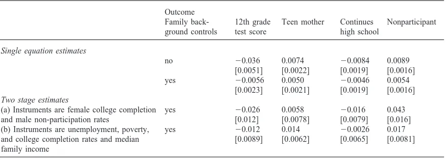
Table 2 presents single equation and instrumental vari-able estimates for all four outcomes. The top two rows demonstrate the well known result that the inclusion of controls for family background and prior achievement reduces substantially the magnitude of peer group effect estimates. The estimated effect on test score decreases

Table 2

Estimated peer group effects (Huber/White adjusted standard errors in brackets) Outcome

Family back- 12th grade Teen mother Continues Nonparticipant ground controls test score high school

Single equation estimates

no 20.036 0.0074 20.0084 0.0089

[0.0051] [0.0022] [0.0019] [0.0016]

yes 20.0056 0.0050 20.0046 0.0054

[0.0023] [0.0021] [0.0019] [0.0016]

Two stage estimates

(a) Instruments are female college completion yes 20.026 0.0058 20.016 0.043

and male non-participation rates [0.012] [0.0078] [0.0079] [0.016]

(b) Instruments are unemployment, poverty, yes 20.012 0.014 20.0026 0.017 and college completion rates and median [0.0089] [0.0062] [0.0065] [0.0081] family income

by over 80 percent while the decreases for the other three outcomes range between 30 and 50 percent. Neverthe-less, the estimates remain statistically significant at the two percent level for all outcomes. Controlling for 10th grade test score, family background and the money and time costs of schooling does not eliminate the relation-ship between the four outcomes and percent disadvan-taged. At the variable means, a ten percentage point increase in percent disadvantaged increases the prob-abilities of being a teen mother and of nonparticipation and decreases the probability of high school continuation all by roughly 2 percentage points. It also reduces 12th grade test score, but by less than one tenth of a stan-dard deviation.

(7)

Specifi-cations that use the female college completion and male nonparticipation rates as instruments all produce peer effect estimates that are larger in magnitude than the sin-gle equation coefficients.16_{Three of the four are also} sig-nificant at the five percent level. This pattern of results is in sharp contrast to that found by Evans, Oates, and Schwab for teen pregnancy and high school continuation, and it provides little support for the strategy of using community characteristics as instruments to reduce the magnitude of endogeneity bias.

Why do these results differ from those of Evans et al. (1992)? One possible explanation is that the estimates are sensitive to the choice of instruments.17_{However, the} final row of Table 2 shows that the IV estimates pro-duced by the Evans, Oates, and Schwab set of instru-ments also tend to be larger than the single equations estimates, including the teen mother specification for which the IV peer effect estimate is large and statistically significant. Only the IV estimate in the high school con-tinuation specification, for which the standard error is very large, is smaller in magnitude than the single equ-ation coefficient.

While the desirability of one set of instruments over the other is a secondary issue, it should be noted that the four instrument set failed the Sargan test at the 10 per-cent level for the test score specification (the only

con-tinuous outcome).18_{Given that the outcomes are highly}

correlated, this suggests that one or more of these instru-ments may be correlated with the structural error in all specifications. The Sargan test statistic is not reported for the first set of instruments because the first stage esti-mate for one of the two instruments was not statistically significant. However, in specifications that use average mother’s education as the peer group measure, both instruments are significant in the first stage, and the hypothesis of no correlation with the structural error is not rejected at the 10 percent level.19_{In any case, a} simi-lar pattern of single equation and IV estimates holds for both sets of instruments.

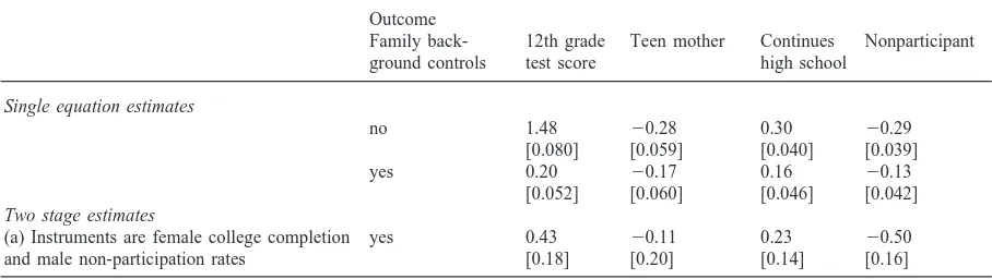
16 _{Appendix B shows that this pattern of results also holds if}

the average education of schoolmates’ mothers is used to meas-ure peer group background.

17 _{Small differences in specification or methodology may also}

contribute to the discrepancy in findings. In particular, Evans et al. (1992) use a more efficient methodology in the estimation of the instrumental variables probit models. They nevertheless obtain much noisier estimates.

18 _{There are three over-identifying restrictions in this}

regression, so the Sargan test statistic has a Chi Square distri-bution with three degrees of freedom. The test statistic equals 6.9 which exceeds the critical value of 6.25.

19 _{The test statistic equals 0.95 which does not exceed the}

critical value of 2.71.

Because Evans, Oates, and Schwab used metropolitan area characteristics as instruments and restricted the sam-ple to students from metropolitan areas, it is also possible that differences in the aggregation level and sample selection criteria account for the discrepancy in results. Table 3 provides single equation and IV estimates for specifications restricted to students from metropolitan area high schools. Similar to Table 2, the metropolitan area level instruments do not systematically reduce the estimated peer group effects. In the test score20_and non-participation specifications, the IV estimates are again larger than the single equation estimates, while for the teen mother specification the IV and single equation esti-mates are virtually identical in size. Finally, for the high school continuation specification the IV estimate is roughly equal in magnitude but opposite in sign to the probit coefficient, and the estimate is quite imprecise. In fact it is the imprecision of the high school continuation and teen fertility estimates that is most similar to the results of Evans, Oates, and Schwab, and such impre-cision provides little if any reason to conclude that the IV estimates reduce endogeneity bias. Importantly, the other two outcomes, nonparticipation in particular, pro-vide much stronger epro-vidence against the argument that aggregation moves the estimates closer to the true value. Thus there is little support for the view that aggre-gation reduces specification error in the estimation of peer group effects. While the teen fertility and high school continuation estimates for residents of metropoli-tan areas are fairly similar across the two studies, the chief commonality is their imprecision. The often stat-istically significant findings for the expanded set of out-comes, instruments and samples provide a pattern of results that contradicts the belief that aggregation ameli-orates problems introduced by the nonrandom sorting of families.

5. Conclusion

The overall pattern of estimates is not consistent with the belief that county group or metropolitan area charac-teristics provide valid instruments for school level data in analyses of peer group effects. Rather, the results sug-gest that aggregation tends to move estimates further from their true values. In combination with the question-able theoretical justification for the use of aggregate data as instruments, the lack of statistical information on instrument validity, and the findings from studies of school resources, this evidence raises strong doubts

20 _{The overidentification test is also failed with the restricted}

(8)

Table 3

Estimated peer group effects for women who attend high school in metropolitan areas (Huber/White adjusted standard errors in brackets)

Outcome

yes 20.0070 0.0070 20.0071 0.0061

[0.0030] [0.0025] [0.0022] [0.0021]

(a) Instruments are unemployment, poverty, yes 20.016 0.0062 0.006 0.036 and college completion rates and median [0.015] [0.0087] [0.0082] [0.014] family income

Table 4

Explanatory power of instruments in first stage regressions of percent disadvantaged on exogenous variables (Huber/White adjusted standard errors in brackets)

(i) Instrument set a

Non-participation rate for men 142.6 [33.6] Proportion of women who are 29.09 college graduates [6.31]

(ii) Instrument set b

College graduation rate 222.6

[10.3]

Unemployment rate 248.9

[38.6]

Poverty rate 144.0

[31.6]

Median family income 0.00069

[0.00030]

F test statistic 10.68 9.33

[2, 756] [4, 756]

Table 5

Estimated peer group effects using average mother’s education of schoolmates as the peer group measure (Huber/White adjusted standard errors in brackets)

Outcome

no 1.48 20.28 0.30 20.29

[0.080] [0.059] [0.040] [0.039]

yes 0.20 20.17 0.16 20.13

[0.052] [0.060] [0.046] [0.042]

(a) Instruments are female college completion yes 0.43 20.11 0.23 20.50

and male non-participation rates [0.18] [0.20] [0.14] [0.16]

about the benefits of aggregation as a method to reduce endogeneity bias.

(9)

hous-ing voucher trials in five different cities.21 _{The results} should provide much needed information about the mag-nitude and importance of peer group effects for different outcomes and demographic groups.

Acknowledgements

I would like to thank Walter Nicholson, Geoffrey Woglom, two anonymous referees, and seminar parti-cipants at the University of Massachusetts for their many helpful comments and the William H. Donner and Smith Richardson Foundations for financial support.

Appendix A

Table 4

Appendix B

Table 5

References

Brown v. Board of Education (1954). 347 US 483.

Card, D., & Krueger, A. (1996). School resources and student outcomes: An overview of the literature and new evidence from North and South Carolina. Journal of Economic

Per-spectives, 10, 31–50.

Case, A., & Katz, L. (1991). The company you keep: The effects of family and neighborhood on disadvantaged youths. National Bureau of Economic Research Working Paper 3705.

Crane, J. (1991). The epidemic theory of ghettos and neighbor-hood effects on dropping out and teenage child rearing.

American Journal of Sociology, 56, 1226–1259.

Coleman, J. et al. (1966). Equality of educational opportunity. Washington, DC: US Department of Health, Education, and Welfare.

Evans, W., Oates, W., & Schwab, R. (1992). Measuring peer group effects: A study of teenage behavior. Journal of

Polit-ical Economy, 100, 966–991.

Grogger, J. (1996). School expenditures and post-schooling

21 _{See Katz, Kling, and Liebman (1997), Ladd and Ludwig}

(1997), and Ludwig, Duncan, and Hirschfield (1998) for pre-liminary evidence on the MTO experiment.

earnings: Evidence from the high school and beyond.

Review of Economics and Statistics, 78, 628–637.

Hanushek, E., Rivkin, S., & Taylor, L. (1996). Aggregation and the estimated effects of school resources. Review of

Eco-nomics and Statistics, 78, 611–627.

Hanushek, E., Kain, J., Markman, J., & Rivkin, S. (1999). Peer

group effects on student achievement. Mimeo.

Jencks, C., & Mayer, S. (1990). The social consequences of growing up poor. In L. Lynn Jr., & M. McGeary,

Inner-city poverty in the United States. Washington, DC: National

Academy Press.

Katz, L., Kling, J., & Liebman, J. (1997). Moving to opportunity

in Boston: Early impacts of housing mobility programs.

Mimeo, Harvard University.

Ladd, H., & Ludwig, J. (1997). The effects of MTO on

edu-cational opportunities in Baltimore: early evidence.

Work-ing paper, Northwestern University/University of Chicago Joint Center for Poverty Research.

Ludwig, J., Duncan, G., & Hirschfield, P. (1998). Urban

pov-erty and juvenile crime: evidence from a randomized hous-ing-mobility experiment. Working paper.

Maddala, G. S. (1983). Limited-dependent and qualitative

vari-ables in econometrics. Cambridge University Press.

Moffit, R. (1995). Selection bias adjustment in treatment-effects models as a method of aggregation. 1995 Proceedings of

the American Statistical Association, 234–238.

Moffitt, R. (1998). Policy interventions, low level equilibria,

and social interactions. Working paper.

Peterson’s Guide to Four Year Colleges (1983). Princeton:

Pet-erson’s Guides.

Rivkin, S. (1995). Black/white differences in schooling and employment. Journal of Human Resources, 30, 826–852. Rivkin, S., & Woglom, G. (1999). Testing the validity of

instru-ments: a cautionary note. Amherst College.

Rosenbaum, J. (1992). Black pioneers—Do their moves to the suburbs increase economic opportunity for mothers and chil-dren? Housing Policy Debate, 2, 1179–1213.

Stinchcombe, A. (1969). Environment: The cumulation of effects is yet to be understood. Harvard Educational

Review, 39, 511–522.

Tiebout, C. (1956). A pure theory of local expenditures. Journal

of Political Economy, 64, 416–424.

US Department of Commerce (1980). Census of Population and

Housing (United States): Public Use Microdata A Sample.

Bureau of the Census, Washington, DC.

US Department of Education, Center for Education Statistics (1986). High School and Beyond, 1980: Sophomore Base

Year, 1st, 2nd, and 3rd Follow-up Surveys. Produced by

National Opinion Research Center.