ROOF RECONSTRUCTION FROM POINT CLOUDS USING IMPORTANCE SAMPLING
William Nguatem, Martin Drauschke, Helmut Mayer
Institute of Applied Computer Science Bundeswehr University Munich
Werner-Heisenberg-Weg 39, 85577 Neubiberg, Germany william.nguatem,martin.drauschke,[email protected]
Commission III/4
KEY WORDS:Building Reconstruction, Point Cloud Segmentation, MCMC, Model Selection, Non-linear Regression Fitting
ABSTRACT:
We propose a novel fully automatic technique for roof fitting in 3D point clouds based on sequential importance sampling (SIS). Our approach makes no assumption of the nature (sparse, dense) or origin (LIDAR, image matching) of the point clouds and further distinguishes, automatically, between different basic roof types based on model selection. The algorithm comprises an inherent data parallelism, the lack of which has been a major drawback of most Monte Carlo schemes. A further speedup is achieved by applying a coarse to fine search within all probable roof configurations in the sample space of roofs. The robustness and effectiveness of our roof reconstruction algorithm is illustrated for point clouds of varying nature.
1 INTRODUCTION
The generation of accurate 3D city models from point clouds is a very active research topic in computer graphics, photogrammetry and computer vision, (Wahl et al., 2008; Huang et al., 2013; La-farge et al., 2013). The main focus of these related contributions has been to achieve (a) a significant amount of data reduction, (b) the automation of object recognition and reconstruction from un-structured 3D point clouds, and (c) the integration of semantics into building and 3D city models. However, most of the efforts in this domain are based on the analysis of terrestrial and airborne LIDAR data sets. The two major reasons for this are (1) the matu-rity of the LIDAR technology and (2) the resulting high accuracy and very dense 3D data.
However, due to the general availability of digital cameras, there is an immense interest in the generation of 3D point clouds from multiple images (Snavely et al., 2006; Frahm et al., 2010; Bar-telsen et al., 2012). Though this data acquisition pipeline is being improved due to the developments of new algorithms for dense matching such as (Strecha et al., 2008; Hirschmueller, 2008; Kuhn et al., 2013), the acquired 3D points are still inferior to data acquired from LIDAR as far as accuracy is concerned. How-ever, the 3D data are good enough to reliably recognize objects and their parts. Furthermore, these algorithms also benefit from the inherent flexibility using a standard consumer camera. We see a trend in an increasing quality of the 3D point clouds from matching and thus a necessity for devising methods for roof re-construction from point clouds, which are robust with respect to the different data acquisition process.
The goal of our work is to find, classify and fit basic roof types above a given quadrilateral building footprint. Thus, we aim at a level-of-detail (LOD) 2 model, consisting of the basic 3D shape such as a gable or a mansard roof. This will act as an interme-diate state in a hierarchical modeling of buildings. A wide vari-ety of applications in robotics, automotive navigation, tourism or city planning can benefit from such an automated building roof reconstruction scheme. We illustrate our algorithm with exper-imental results for data from matching images. We employ ter-restrial images combined with images obtained from unmanned aircraft system collected in Southern Germany. Additionally, LI-DAR data sets and synthetic data sets generated from sampling a
CAD model with additive noise are used in our experiments. The paper is structured as follows. Section 2 discusses existing approaches for reconstructing roofs in 3D point clouds. Begin-ning with an overview, we present our algorithm in Section 3. This is followed by the discussion of experimental results in Sec-tion 4. In SecSec-tion 5, we conclude and give direcSec-tions for future work.
2 RELATED WORK
There is a significant amount of work on the reconstruction of building roofs from point clouds. Most often, this is done based on domain knowledge, e.g., using shape priors of the objects of interest (Huang et al., 2013). Sampath and Shan (2010) take cur-vature as a feature within a fuzzy k-Means framework to cluster points defining roof segments in aerial LIDAR data. A similar re-gion growing approach (Rottensteiner, 2010) detects planar sur-faces by combining information from multiple images and point clouds. These surfaces can further be classified into various roof types. A Markov Chain Monte Carlo (MCMC) approach to roof reconstruction is presented in (Huang et al., 2013). Here, sam-ples of possible roof constellations are proposed from within a predefined library of planar shapes. Proposals may or may not be accepted within a Reversible Jump MCMC (RJMCMC) setting depending on their computed likelihoods. However, the genera-tive nature of the algorithm makes it very sensigenera-tive to noise and the RJMCMC sampler means a bad scalability of the algorithm. In (Taillandier and Deriche, 2004), a bayesian approach is used to fit polyhedral models from aerial images. The resulting planar patches are used to construct graphs from which buildings are reconstructed.
Figure 1: At each height level, the configuration with the high-est likelihood is marked in bold. The black arrows describe the transition of the configurations from one level to the next and the gray dots are data points. Different colors correspond to different configurations. Please note that the space between height levels is widely exaggerated for a better comprehension.
that can cope with very sparse data sets. It assumes an underlying rectangular footprint. M-estimator random consensus (MSAC) proposed by Torr and Zisserman (2000) is used as a robust esti-mator to fit basic roof models. To differentiate between compet-ing roof types, a support vector machine was used for classifica-tion. However, the approach is not suited for point clouds from image matching which are often highly irregular distributed and more complex roofs (mansard, gambrel etc.). Additionally, the assumption of a perfect rectangular footprint may be too strong a constraint. Besides the above mentioned deficits the majority of the mentioned algorithms are tailored for LIDAR data sets. Our algorithm contains an extension of the parametrization of (Poullis and You, 2009), combined with a likelihood model simi-lar to (Henn et al., 2013) within a Monte Carlo (MC) setting sim-ilar to (Huang et al., 2013), to optimally explore the search space for roof types above a detected general quadrilateral footprint.
3 PROPOSED METHOD
3.1 Overview of the Algorithm
The input to our system is an unstructured 3D point cloud,D, containing a building as viewed from outside and above. The output is a set of connected polygonal surfaces above a general quadrilateral footprint with a defined roof type, e.g., mansard, gable or pinnacle. We suppose the 3D region above the footprint defines the most plausible search space for a roof. Appropriately, we transformDto a coordinate frame where the direction vec-tor(0,0,1)points upwards. Starting at the highest point above the footprint and descending in discrete steps, we estimate prob-ability distributions over possible roof configurations at several height levels. Making no assumptions about the form of these probability distributions over roofs at each level, our objective is to find the configuration that “best” explainsD.
In Fig. 1, we show a gable roof illustration of this probabilis-tic roof fitting scheme using four roof configurations (coloured black, green, blue and yellow) and three height levels (l0,l1,l2).
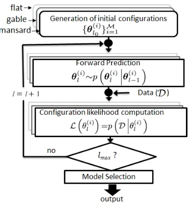
Figure 2:Roof fitting using sequential importance sampling.
First, we build initial roof configurations (levell0) and estimate their likelihoods. Then, iteratively a transition is made to the next level and the roof configurations likelihood is updated. At each level, the configuration with the highest likelihood (marked bold in Fig. 1) explains our data better than all other configurations present. At height levell2, configurationθ1(black in Fig. 1) pro-vides a better fit than all other configurations. The problem is de-fined in a Bayesian setting and a sequential Monte Carlo (SMC) approach is used to search for a solution.
3.2 Notation
Random pointspjare considered in the subspaceΦ∈R3of the 3D Euclidean space. An ordered sequenceθ ≡ (p1· · ·pq) ∈
Φq uniquely defines a 3D surface in some standard way, e.g., in our experiments the p’s are the vertices of a 3D polygonal chain.Thus,θrepresents a single roof configuration. The sym-bollrepresents a discrete height level index. Pldefines a plane with normal vector(0,0,1), passing through height levell. The symbol∼means “distributed according to” as inx∼ N(m, σ2) defining the Gaussian random variablexwith meanmand stan-dard deviationσ andy ∼ U(a, b) refers to a uniform random variableywith support[a, b]. Draws are collected, unless other-wise stated, in an independent and identically distributed (i.i.d.) way. The same notation will be used for a random variable and its realization to reduce notational clutter.
Being in an MC setting, we use a set of discrete roof configura-tions to approximate a distribution over roofs. For example, at levell,{θ(i)l }M
i=1are a finite set ofMsuch 3D polygonal chains used as a discrete representation ofp(θl|D), the distribution over polygonal chains at levell. The likelihood of a configuration, L(θ(i)l ), denotes how the data is explained by that polygonal chain. The normalized likelihood defines the weight of a config-uration,w(i)l . This is used as an approximation of the posterior probability,p(θ(i)l |D). At each height level, the configuration with the highest weight is reckon on as the maximum a-posteriori probability (MAP) configuration, denotedθM AP (bold lines in Fig. 1).
3.3 Roof Fitting using a Sequential Monte Carlo Method
levels along the vertical direction, we employ sequential impor-tance sampling (SIS) to consistently keep track of roof configu-rations at these height levels. This iteratively approximates the distribution over roof configurations. The goal is to move the starting configurations based on a forward transition distribution,
p(θl|θl−1), which retains expected properties of the 3D polygo-nal chains to be fitted and on an observation model,p(D|θl), that provides evidence about whether a measured 3D point inDis in the close vicinity of the “true” 3D polygonal chain. The com-plete algorithm summarized in the flow chart given in Fig. 2 can be described as follows:
1. In initialization, we generate Mconfigurations for every considered roof type (mansard, gable, flat, etc.)
2. In forward prediction, theseMconfigurations per roof type are propagated using the transition probability distribution,
p(θl|θl−1). This results in a change of configurations from one level to another
3. Within an update stage, likelihoods of the configurations, Lθ(i)l , are estimated and normalized, thus giving a dis-crete approximation of the posterior probability,p(θl|D)
4. Steps 2 and 3 are iterated until a minimum level well above the ground plane (denoted bylmaxindex) is reached
5. At the minimum level, we are confronted with three prob-lems: (1) Which of the considered roof types explains our data better than the others? (2) Amongst the levels, which posterior distribution,p(θl|D), should be chosen? (3) Con-sidering all theMconfigurations accounting for the chosen posterior distribution, which configuration explains our data “best”?
We divide the above algorithm into four major parts: Initializa-tion, forward predicInitializa-tion, weight estimation (roof configuration likelihood estimation) and model selection. Details of these ma-jor parts of our algorithm are described in the following.
3.3.1 Initialization The generation of initial configurations means to choose an appropriate parametrization for the vari-ous basic roof types and corresponding prior distributions for them. We could extend the generic mansard roof parametriza-tion of (Poullis and You, 2009) to include all symmetric and asymmetric variants of these basic roof types. However, this would be too computational intensive for a scene with few mansard roofed buildings. Therefore, we have devised more distinctive parametrization for different types of roofs. We use non-informative priors for the parameters defining the building heights,p0,p1,p2,p3in Fig. 3 and Fig. 4. This prior compen-sates for uncertainty in the estimates of heights of the buildings walls. Therefore, for the pointsp0,p1,p2,p3, we make four i.i.d. draws given by
p(i)∼ U(pk−0.5hd,pk+ 0.5hd), (1)
wherek ∈ {0,1,2,3}stands for the respective pointspk, hd is the height tolerance as depicted in Figs. 3 and 4 and iis the index of thei-th ofMconfigurations. Since the direction vector(0,0,1)has been defined as the vertical direction of the scene, equation (1) means a 1-dimensional search along thez -axis. These four draws representing a prior over the height of the walls are fundamental for all roof types.
In addition to equation (1), we use domain knowledge and de-rive informative priors over the ridges, peaks, hips etc. to give a complete prior for a certain roof type.
Figure 3:Top row: gable roof model including variance in build-ing heights (hd) and ridge position (ht). Bottom row: Pinnacle roof model showing hip intersection point tolerance circle with diameterhc.
Figure 4: Top row (a), (b) and (c): Illustration of mansard roof parametrization. Bottom row: In (d) the gray region illustrates the actual search space for the mansard roof excluding pinnacle roof candidates. (e) and (f) illustrate the symmetric and asym-metric (half)-hipped roof parametrization respectively.
Gable Roof PriorFig. 3 illustrates the parametrization of the gable roof. A prior over the ridge combined with equation (1) defines our informative prior model for the gable roof type. A realization of the ridge is defined by the line segment between pointspraandprbprojected on planePl, where
p(i)ra∼N pma,ht
and p(i)rb∼N pmb,ht
(2)
withpma = 0.5·(p0 +p1)andpmb = 0.5·(p2+p3), ht defines the tolerance in the ridge andiis the index of thei-th configuration. These are 1-dimensional draws along the direction of the walls. Since Equations (1) and (2) are i.i.d. samples, this prior model for the gable roof captures the complete family of gable roofs (symmetric and asymmetric). It is constructed twice such that in each case, the two sloping roof planes are oriented according to wall pairs. This ensures the right orientation of the roof planes to the pair of opposite walls.
realiza-tion of the peak is defined by
p(i)peak∼ N(pmid, hc) (3)
withpmid= 0.25·(p0+p1+p2+p3)the centroid of the four points defining the footprint,hcis the tolerance of the intersection point of all four hips andiis the configuration index. ppeakis projected onPlto get the true peak.
Mansard RoofSimilarly, Fig. 4 shows the parametrization of the mansard roof.
h(i)mlength∼ U(0, hn), h(i)mwidth∼ U(0, hm) (4)
wherehnandhmare tolerance values defining the lengths of the ridges and again,iis the index representing thei-th configuration. The true ridges are a projection of the line segmentsh(i)mwidthand
h(i)mwidthonPl. If the outcome of Equation (4) lies within a circle with diameterhc (cf. Fig. 4d),i.e., a highly probable pinnacle roof candidate, it is rejected. The final valid search space for mansard roof is marked gray in Fig. 4d.
Other Roof TypesThe most basic roof types are the flat and shed roofs. Their parametrization is obtained by varying the four points defining the building height, i.e., equation (1). Figs. 4e and 4f shows our template for the general family of hipped roofs, symmetric, asymmetric and (half)-hipped. Obviously, from this template the parametrization is obtained by a combination of gable and mansard roofs. To increase the effective number of samples and avoid “inverse” and thus invalid roof types, a con-straint is added to all parameterizations that guarantees the ridge being higher than the building walls.
3.3.2 Forward Prediction In Fig. 2, we describe the move-ment of roof configurations from one height level to another as sampling from a forward transition distribution,p(θl|θl−1)given by the following simple first-order model
θ(i)l ∼θ(i)l−1 (5)
Having present the initialization and the forward transition prob-ability, we now proceed to present how the configuration likeli-hoods of the 3D polygonal chains are computed.
3.3.3 Roof Configuration Likelihood Computation We use MSAC (Torr and Zisserman, 2000) to determine if a point inD is within the close vicinity of a 3D polygonal chain defined by a configuration,θ. MSAC underlies a likelihood function propor-tional to a truncated Gaussian bounded by the RANSAC thresh-old,T2. Henn et al. (2013) used a similar likelihood model on aerial LIDAR data. Yet we optimally explore the configuration space in a Bayesian setting. Thus at levell, for a certain config-uration,θ(i)l , assuming measurements being conditionally inde-pendent, the likelihood function is given by
Lθl(i)∝exp (−X
ande2jthe shortest Euclidean distance from pointpjto the sur-face of the 3D polygonal chain defined by the configurationθ(i)l . The summation indexjruns over all the points inD.
3.4 Model Selection
Equation (6) defines the likelihood for a single configuration of a specific roof type. We define the configuration weightw, as the
normalized likelihood, given by
Therefore, the posterior probability at levellfor a roof type is approximated by
whereδ()defines the Dirac function. So far, three major ques-tions are unanswered: (1) the roof type to choose (2) the height level to select and (3) within the chosen height level and roof type, the configuration that fitsD“best”. For the first two questions, we compare weights of the MAP configurations at each level for all the competing roof types and select the roof type whoseθM AP has the highest weight. The height level within which the se-lected,θM APresides defines the selected height level and is used to answer the third question. For this, we adopt theM-opened modelling perspective (Smith and Bernardo, 2000) i.e., we be-lieve the “best” configuration may not be within theM configu-rations of the selected height level for the chosen roof type, how-ever, through Bayesian model averaging, we compute the mini-mum mean square error estimator (MMSE) configuration as the inferred “best” configuration. For the chosen roof type within the selected height level, this is given by
ˆ
The MMSE estimator in this setting is analogous to taking a weighted least square fit with the weights proportional to the es-timated likelihoods as defined in section 3.3.3.
4 EXPERIMENTS
4.1 Implementation Details
The major computational bottleneck is Equation (6), since the likelihood has to be estimated Mtimes per roof type for ev-ery level. To speed up this compuation, we use a coarse to fine search. FirstDis downsampled using a voxel grid with leaf size 0.4m×0.4m×0.4mdefining the input point density. A search is conducted with a large enough inter-height level value to cap-ture the height level where the roof most probably lies. Around the selected level, we apply a finer inter-level value for the final search. We also use a fast version of the polygon hit test from (Schneider and Eberly, 2002) for the various polygon segments of a 3D polygonal chain defining a configuration. Furthermore, since the heights of walls of a building are correlated, a pair-wise sampling of the building height priors was prefered to four i.i.d. draws of Equation (1). In our formulation of SIS, a strong data parallelism is implied due to the 3D space partitioning in dis-crete height levels. Using alternative sampling schemes such as Gibbs, Metropolis-Hastings or sequential importance resampling samplers, this proper decoupling of samples from one level to another is impossible.
4.2 Parameters and Data Sets
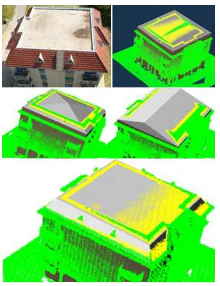
Figure 5: MMSE fit for flat, pinnacle, gable and mansard roof types on a mansard roofed building data set obtained from im-age matching. The yellow points are the inliers to the “best” 3D polygonal chain. As expected, the mansard roof model explains the data best by providing the best fit.
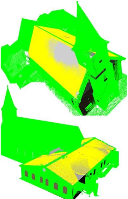
Figure 6: Top row: Image and MMSE fit using a gable roof type. The model is viewed from inside the building. Bottom row: MMSE fit using a pinnacle roof model. The model is viewed from outside (left) and inside (right) the building.
Dataset (roof type) # footprints correct wrong
Laser (gable) 10 10 0
Matching (gable) 5 5 0
Synthetic (gable) 105 101 4
Laser (hipped) 5 5 0
Matching (hipped) 1 1 0
Synthetic (hipped) 15 14 1
Laser (pinnacle) 0 0 0
Matching (pinnacle) 1 1 0
Synthetic (pinnacle) 7 7 0
Laser (mansard) 0 0 0
Matching (mansard) 1 1 0
Synthetic (mansard) 3 3 0
Table 1: Results of our experiments conducted on different data sets. The number of correct versus wrong fits given the footprints.
Parameter T M hc ht hd
Value 0.3m 1000 0.5m 0.5m 2m
For the mansard roof type,hnandhmwere both chosen to be0.5 meters less than length and width of the footprint. Furthermore, we discretized the search space above the footprint in10and5 equal steps for the coarse and the fine search respectively.
Example outputs from data set obtained from image matching is shown in Figs. 5 and 6. For Fig.5, a combination of images taken from the ground and a UAV were used for matching and the mansard roof type best explains the data set. Meanwhile Fig. 6, shows a highly unequal point distribution in the data set with very few points on the roof as a result of the matching of images taken from the ground alone. We were still able to get the pinnacle roof type as the best fitted model. Since synthetic data sets are more or less perfect, for all experiments, all points were perturbed using
pj∼pj+uj (11)
whereuj∼ N(0,1m)for evaluation purpose.
4.3 Results
We tested our algorithm on a data sets containing 152 quadrilat-eral footprints of 3D points of varying density and origin. The results is summarized in the Table 1. All wrongly fitted roofs re-sulted in a flat roof type. This was due to the very low inclination angle of the roof planes. However, by tuning the parameters one can certainly get rid of these inaccuracies in the fits.
4.4 Clutter
Figure 7: Data from LIDAR with a T-shaped building footprint decomposed into two separate non-overlapping quadrilaterals. The yellow points are the inliers of the MMSE fitted roof type over each footprint. Best fit in spite of substantial clutter
Secondly, the choice of the likelihood and the proper exploration of the search space within a Bayesian setting provides the optimal fit in MMSE sense.
5 CONCLUSION
We presented a sampling based method for automatically fitting and classifying building roof models from 3D point clouds. As-suming a general quadrilateral footprint, the method starts with the construction of parametric models of different roof types. These are represented by an ordered sequence of 3D polygo-nal surfaces. A likelihood function is chosen that considers the closeness of the 3D Data to the 3D polygonal chains. These likelihoods are used within a Bayesian setting to build proba-bility distributions for various roof types in several possible dis-crete height levels above the footprint. Using model averaging, a model selection scheme is chosen to get the “best” model in MMSE sense. We achieve a computational speedup by applying a coarse to fine search. The method yields geometrically accu-rate parametric building roof models and is robust concerning the source and nature of the input data. For the generic case of mod-eling 3D buildings with a quadrilateral footprint, our approach robustly produces reliable results from which further refinements can be made, progressively increasing the level of detail towards detailed model (LOD3). A parametric representation is chosen which directly encodes to state-of-the art visualization and rep-resentation environments such as CityGML. Practical problems arise particularly due to extreme occlusions and wrong priors. To
overcome this problem, it would be desirable to extend the likeli-hood function.
References
Bartelsen, J., Mayer, H., Hirschm¨uller, H., Kuhn, A. and Miche-lini, M., 2012. Orientation and Dense Reconstruction from Unordered Wide Baseline Image Sets. PFG (4), pp. 421–432.
Frahm, J.-M., Fite-Georgel, P., Gallup, D., Johnson, T., Raguram, R., Wu, C., Jen, Y.-H., Dunn, E., Clipp, B., Lazebnik, S. and Pollefeys, M., 2010. Building Rome on a Cloudless Day. In: ECCV, LNCS 6314, pp. 368–381.
Henn, A., Gr¨oger, G., Stroh, V. and Pl¨umer, L., 2013. Model Driven Reconstruction of Roofs from Sparse LIDAR Point Clouds. ISPRS Journal of Photogrammetry and Remote Sens-ing 76, pp. 17 – 29.
Hirschmueller, H., 2008. Stereo Processing by Semiglobal Matching and Mutual Information. PAMI 30(2), pp. 328–341.
Huang, H., Brenner, C. and Sester, M., 2013. A Generative Statis-tical Approach to Automatic 3D Building Roof Reconstruction from Laser Scanning Data. ISPRS Journal for Photogramme-try and Remote Sensing 79, pp. 29–43.
Kuhn, A., Hirschm¨uller, H. and Mayer, H., 2013. Multi-Resolution Range Data Fusion for Multi-View Stereo Recon-struction. 35th GCPR, Saarbr¨ucken, Germany.
Lafarge, F., Keriven, R., Bredif, M. and Vu, H.-H., 2013. A Hy-brid Multi-View Stereo Algorithm for Modeling Urban Scenes. PAMI 35(1), pp. 5–17.
Poullis, C. and You, S., 2009. Photorealistic Large-Scale Urban City Model Reconstruction. IEEE Transactions on Visualiza-tion and Computer Graphics 15(4), pp. 654–669.
Rottensteiner, F., 2010. Roof Plane Segmentation by Combin-ing Multiple Images and Point Clouds. In: The International Archives of the Photogrammetry, Remote Sensing and Spatial Information Sciences, Vol. XXXVIII, pp. 245–250.
Sampath, A. and Shan, J., 2010. Segmentation and Reconstruc-tion of Polyhedral Building Roofs From Aerial Lidar Point Clouds. IEEE Transactions on Geoscience and Remote Sens-ing 48(3), pp. 1554–1567.
Schneider, P. and Eberly, D., 2002. Geometric Tools for Com-puter Graphics. Morgan Kaufmann.
Smith, A. and Bernardo, J., 2000. Bayesian Theory. Wiley Series in Probability and Statistics, Wiley.
Snavely, N., Seitz, S. M. and Szeliski, R., 2006. Photo Tourism: Exploring Photo Collections in 3D. ACM Transactions on Graphics 25(3), pp. 835–846.
Strecha, C., von Hansen, W., Van Gool, L., Fua, P. and Thien-nessen, U., 2008. On Benchmarking Camera Calibration and Multi-View Stereo for High Resolution Imagery. In: CVPR.
Taillandier, F. and Deriche, R., 2004. Automatic Builings Recon-struction from Aerial Images : a Generic Bayesian Framework. In Proceedings of the XXth ISPRS Congress, Istanbul, Turkey.
Torr, P. H. S. and Zisserman, A., 2000. MLESAC: A New Ro-bust Estimator with Application to Estimating Image Geome-try. CVIU 78(1), pp. 138–156.