The influence of management characteristics on the technical
efficiency of wheat farmers in eastern England
Paul Wilson
a,∗, David Hadley
b, Carol Asby
caDivision of Agriculture and Horticulture, The University of Nottingham, Sutton Bonington Campus, Loughborough, LE12 5RD, UK bSchool of Geography and Environmental Sciences, The University of Birmingham, Edgbaston Birmingham, B15 2TT, UK
cRural Business Unit, Department of Land Economy, The University of Cambridge, Cambridge, CB3 9EP, UK
Received 24 August 1999; received in revised form 2 March 2000; accepted 11 April 2000
Abstract
Technical efficiency of wheat farms in eastern England is measured through the estimation of a stochastic frontier production function using panel data for the 1993–1997 crop years. Variations in the technical efficiency index across production units are explained through a number of managerial and farm characteristic variables following Battese and Coelli (1995) [Empirical Econ. 20, 325–332] and incorporating the spirit of Rougoor et al. (1998) [Agric. Econ. 18, 261–272]. The technical efficiency index across production units ranges from 62 to 98%. The objectives of maximising annual profits and maintaining the environment are positively correlated with, and have the largest influence on, technical efficiency. Moreover, those farmers who seek information, have more years of managerial experience, and have a large farm are also associated with higher levels of technical efficiency. Future studies that seek to explain variation in technical efficiency should include further aspects of the managerial decision-making process. © 2001 Elsevier Science B.V. All rights reserved.
Keywords: Technical efficiency; Managerial capacity; Wheat yields
1. Introduction
Numerous studies have identified wide variation in the physical and financial performance achieved by farmers and farm managers operating within the same environmental and economic constraints. Kay and Edwards (1994) argue that in many instances this difference in performance is due to variation in management. However, unlike land, labour and capital, management is not directly observable; sub-sequently this complicates any analysis that attempts to explain the influence of management on farm
per-∗Corresponding author. Tel.:+44-115-951-6075; fax:+44-115-951-6060.
E-mail address: [email protected] (P. Wilson).
formance. Kay and Edwards define the functions of management as planning, implementation and con-trol. Rougoor et al. (1998) have renewed the debate on how to measure the ability of a farmer to influence his/her farm results. Rougoor et al. (1998) broadened the definition of management and group management capacity into two components: personal aspects (e.g. drives, motivations, abilities and biographical facts) and aspects of the decision-making process (e.g. the practices and procedures in planning, implementa-tion and control of decisions). It is argued that these two components are linked because the personal as-pects of the manager may influence his/her ability to follow a decision-making process. Moreover, ac-counting for only one of these two components is argued to be a necessary but not sufficient condition
if management is to be measured correctly. Rougoor et al. (1998) argue that a manager may possess high personal skills yet fail to achieve high performance if the decision-making process is poor. Following a well-defined process helps a decision-maker to make a decision in a logical and organised manner that will, on average, lead to better results (Rougoor et al., 1998).
Empirical studies that seek to quantify the influence of management on farm technical performance gener-ally attempt to explain variation in technical efficiency as a function of management ability through the in-clusion of biographical variables in the analysis (e.g. Battese et al., 1996). Such studies have gone some way towards quantifying the impact of management on farm performance yet are open to the criticism that they ignore aspects of the decision-making process as defined above. Other studies conclude that to gain a greater understanding of the influence of management requires more detailed information about management decision-making and ability in addition to biograph-ical data (Wilson et al., 1998). Rougoor et al. (1998) reinforce this view and conclude that a logical next step in defining farmers’ management capacity would be to include aspects of the decision-making pro-cess when explaining variation in technical efficiency levels amongst farmers.
The focus of this study is to explain the influence of management on the technical performance of wheat farmers in eastern England. The study differs from much previous research into the estimation and expla-nation of technical efficiency by including variables that relate to both personal aspects and aspects of the decision-making process of the farmer as suggested by Rougoor et al. (1998). The data used in this re-search are taken from two related sources: production data collected as part of a study into the economics of cereal production and an attitudinal questionnaire collected specifically to obtain data on aspects of managerial capacity.
The structure of the paper is as follows. Section 2 describes the surveys from which the data sample analysed is derived and defines and provides summary statistics for the variables that enter the model. In Sec-tion 3 the inefficiency effects model is specified and empirical results from this are presented and discussed in Sections 4 and 5. The final section summarises the findings of this research.
2. The data
Cereal production in Great Britain is concentrated in eastern England. The climate of eastern England is favourable to arable rather than livestock production, and subsequently, the eastern region of England con-tains nearly 50% of the cereal area of Great Britain (MAFF, 1997). For this reason the data used in this study are drawn from this region of England.
Table 1
Mean annual values for yield and inputs, 1993–1997a Year No. of
farms
Yield (tonnes/ha)
Seed (£/ha)
N P K (kg/ha)
Crop protection (£/ha)
Labour (h/ha)
Machinery (h/ha) 1993 71 8.04 (1.37) 51.20 (12.18) 270.40 (95.61) 99.92 (26.45) 9.46 (2.69) 139.74 (35.94) 1994 72 7.96 (1.31) 54.70 (14.45) 278.49 (75.39) 99.35 (26.99) 9.46 (2.67) 139.00 (36.24) 1995 72 8.15 (1.19) 44.37 (10.72) 288.60 (70.81) 106.23 (31.86) 9.39 (2.59) 139.12 (36.15) 1996 74 8.38 (1.22) 42.26 (9.14) 285.93 (75.55) 104.50 (27.62) 9.43 (2.65) 138.23 (36.05) 1997 73 7.96 (1.48) 47.20 (10.72) 277.18 (67.63) 107.16 (31.48) 9.46 (2.65) 138.07(36.27) Total obervations=362
aStandard deviations shown in parentheses. Labour and machinery data based on 1993 per ha utilisation (annual averages differ due
to changes in the number of observations, and the composition of the sample in each year).
data (both being measured in terms of the hours of each that were applied to the wheat crop) are only available for 1993 we assume that per ha utilisation of these inputs remains fixed over the period.
In order to provide a consistent measure of output (since the sampled farms produced a wide variety of grades of wheat) feed wheat equivalents were derived by first calculating the mean annual price for feed wheat within the sample and then dividing this price into the gross return for wheat of all qualities on each farm. Table 1 gives a broad description of the data, showing changes between 1993 and 1997. Yield is calculated from the total tonnes produced per farm as tonnes of feed wheat equivalent per ha of wheat area. Inputs are given per ha of wheat area, as costs for seed and crop protection, as kilograms for fertiliser and in hours of labour and machinery use. The cost of seeds was used to capture differences in quality of purchased and farm-saved seed (for which physical units were not available). Both seed and crop protection costs are de-flated using appropriate indices to 1993 prices.1 The number of farms included in the panel data set varies slightly from year to year because a small number of farmers in the set did not grow wheat in every year considered.
Table 1 shows the means and standard deviations for outputs and inputs for the years 1993–1997 for this sample. Note that yield, seed costs and crop protec-tion costs have remained fairly stable over the 5-year
1The seed deflator is from the MAFF Index of purchase prices of
the means of agricultural production. The crop protection deflators (which are detailed by type, e.g. herbicides, fungicides, etc.) were supplied by MAFF York (Branch A, Market Prices, Stats C&S).
period. Fertiliser application showed more variation with usage increasing in 1995 and 1996 and falling again in 1997.
Variation in levels of input use among farms for each year is relatively small. This is possibly due to farmers applying these inputs following recom-mended application rates per ha (where manufactur-ers and/or advisors make recommendations). Given this small variation in application rates we would expect that efficiency differences among farms are also likely to be small and that these differences will be explained by either factors which remain beyond control of the farmer, e.g. climatic and locational variations (which are not explored here because of data limitations) or differences in the management input on each farm. This small variation in appli-cation rate also raises issues for model formulation. Variables defined as annual levels of inputs were found to be very highly collinear with land area and each other (with correlation coefficients of 0.9 and above), hence the variables which enter the stochastic frontier production function analysis are defined on a per ha basis in an attempt to mitigate multicollinear-ity problems. This problem is common in empirical agricultural production analysis although it is particu-larly acute in this case where single enterprise (rather than whole farm) data is utilised. The implications of using a yield function, rather than the more conven-tional production function, are discussed further in Section 3.2.
Table 2
Definition of variables hypothesised as influencing technical efficiency Variable Definition
AREA Total area of each farm (ha) EXP No. of years of managerial experience
FED Dummy variable=1 if decision maker has had some form of higher education (diploma, degree, etc.) and 0 otherwise PMAX Dummy variable=1 if farmer ranks profit maximisation as 1 or 2 in answer to business objectives
ENV Dummy variable=1 if farmer ranks maintaining the environment as 1 or 2 in answer to business objectives INFSEEK Number of information sources the farmer utilises of the 16 listed in the questionnaire
TIME Linear time trend (1=1993 to 5=1997)
produced the sample of 74 farms for which production data is summarised in Table 1. The face-to-face inter-views specifically asked farmers about their number of years of managerial experience, whether they had undertaken further education, their use of advisors and consultants and their methods of acquisition of technical information. In addition, the farmers were asked to rank in order of importance to them the fol-lowing four business objectives: maintain way of life, maximise annual profits, maintain environment and increase farm size/business.
From the responses received, a number of variables were formulated which were hypothesised as possi-bly having a role in explaining differences in levels of technical efficiency among farms. Definitions of these variables are outlined in Table 2, while Table 3 provides summary statistics.
Of the variables defined in Table 2, experience, further education, profit maximisation and maintain-ing the environment relate to the personal aspects of managerial capacity as defined by Rougoor et al. (1998). Of these, the first two can be considered as biographical characteristics whilst the latter relate to
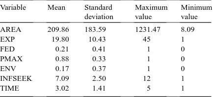
Table 3
Summary statistics for variables hypothesised as influencing tech-nical efficiency, 1993–1997
Variable Mean Standard deviation
Maximum value
Minimum value AREA 209.86 183.59 1231.47 8.09
EXP 19.80 10.43 45 1
FED 0.21 0.41 1 0
PMAX 0.88 0.33 1 0
ENV 0.17 0.37 1 0
INFSEEK 7.09 2.50 12 1
TIME 3.02 1.41 5 1
the drives which motivate farm decision-makers. To capture aspects of the decision-making process, farm-ers were asked to identify from where they obtained technical information about crop husbandry practices from a list of 16 possible sources grouped into four categories as follows:
1. personal: independent advisor, merchant’s advisor, other farmers, others;
2. written: farming press, MAFF literature, Home-Grown Cereals Authority (HGCA) literature, commercial literature, others;
3. electronic: internet, others;
4. others: HGCA conferences, other conferences, local agronomy groups, farmer meetings, others.
An ‘information seeker’ variable was constructed by summing the number of these 16 sources that farmers stated as using. This measure provides an indication of practices and procedures in planning and will have a direct influence on implementation and control of decisions or aspects of the decision-making process in general.
Table 3 shows that the average number of years of managerial experience was approximately 20. Only 21% of the sample had undertaken further education, 88 and 17%, respectively, ranked maximising annual profit and maintaining the environment as one or two in their ranking of objectives, whilst an average of seven information sources, of the 16 listed, were used by farmers.
over this period this does not seem an unreasonable assumption to make.
3. Technical inefficiency effects model and specification
3.1. Model
The Battese and Coelli (1995) technical ineffi-ciency effects model is an extension of the more usual stochastic error component frontier function which allows for identification of factors which may explain differences in efficiency levels between observed decision-making units. The conventional stochastic frontier approach involves estimation of a function with a composite error term, including a symmetric and a one-sided component (following Aigner et al. (1977) and Meeusen and van den Broeck (1977)). In the case of the frontier production function, the symmetric component represents random variations in production due to factors outside the control of the farmer (such as climate, measurement error, etc.) and is assumed to be independently and identically distributed as N(0,σ2). The one-sided component is associated with technical inefficiency of production and measures the extent to which observed output deviates from potential output given a certain level of inputs and technology. Commonly it has been assumed that this component has an identical and independent half-normal distribution, although a va-riety of other distributional specifications are possible (Greene, 1997). A detailed review of the approach can be found in Greene (1997).
The model proposed by Battese and Coelli (1995) builds upon Kumbhakar et al. (1991) and Reif-schneider and Stevenson (1991) and extends to panel data the work of Huang and Liu (1994) who for-mulated a non-neutral stochastic frontier production function model, for cross-sectional data, in which the one-sided inefficiency effects are specified as a function of firm-specific factors and input variables, believed to influence technical inefficiency. The tech-nical inefficiency effect, for the i-th firm in the t-th time period,uit, is defined by the truncation (at zero) of the N(µit,σu2) distribution where the firm specific mean,µit, is specified as follows:
µit=δ0+δ′zit (1)
where zit is a column vector of technical inefficiency explanatory variables and theδs are unknown param-eters which are to be estimated.
3.2. Specification
Following the recommendation of Battese and Broca (1997) we employ a general specification for the model as a starting point and test for sim-pler formulations within a formal hypothesis testing framework. Hence the stochastic frontier production function is specified here as a translog function with the following initial form,
lnyit=α0+
where ln denotes natural logarithms, yit represents wheat yield for the i-th farm in the t-th year, x1 is expenditure (£) per ha on seeds, x2 the kilograms of plant nutrients per ha, x3 the cost of crop protection products per ha, x4 the hours of labour per ha, x5 the hours of machinery per ha, t the linear time trend (1993=1,. . ., 1997=5), v the random error which is assumed independent and identically distributed
N(0,σv2), and αs the parameters to be estimated. The technical inefficiency effects, uit, are defined in Eq. (1) where the z variables correspond to those listed in Table 2.
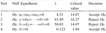
Table 4
Generalised likelihood ratio tests of hypotheses for parameters of the stochastic frontier production function and inefficiency effects modela
Test Null hypothesis λ Critical value
Decision 1 H0:αt=αt t=αkt=0 4.53 14.07 Accept H0
2 H0:γ=δ0=· · · =δ7=0 93.49 16.27 Reject H0
3 H0:δ1=δ2=· · · =δ7=0 50.05 14.07 Reject H0
4 H0:δ7=0 0.123 3.84 Accept H0 aAll tests performed at 5% significance.
to reject the null hypothesis that the sum of production elasticities was greater than or less than one.2
The unknown parameters of Eqs. (1) and (2) in addition to σv2 and σu2 can be estimated simultane-ously using maximum-likelihood — see Battese and Coelli (1993) for details of the likelihood function.3 Predictions of technical efficiency (TE) are calculated according to the following expression:
TEit=exp(−uit). (3)
These predictions are made using the conditional expectation of Eq. (3), given the composed error (vit−uit) and evaluated using the estimated parame-ters presented in Section 4 (Jondrow et al. (1982) and generalised by Battese and Coelli (1988)).
4. Results
4.1. Hypothesis tests and parameter estimates
The model parameters are estimated using the FRONTIER 4.1 program (Coelli, 1996). The pre-ferred model results from the outcome of a sequence of hypothesis tests that are detailed in Table 4.4
2However, given the multicollinearity problems associated with
estimation of this function the results of this test must be treated with some caution.
3The likelihood function is expressed in terms of the variance
ratioγ ≡σ2
u/σs2, whereσs2≡σu2+σv2.
4These are undertaken using the likelihood ratio test. This has
the formλ=2(ln L1−ln L0) where ln L0is the value of the log
like-lihood under the null hypothesis and ln L1the corresponding value
under the alternative hypothesis. It has an approximate chi-square distribution with degrees of freedom equal to the number of independent constraints (Judge et al., 1985).
The first null hypothesis (Test 1) is accepted, indi-cating that no statistically significant technical change occurs in the sample over the period. Test 2 explores the null hypothesis that each farm is fully technically efficient and hence that systematic technical ineffi-ciency effects are zero.5 This is strongly rejected, as is the following null hypothesis which tests whether the variables included in the inefficiency effects model have no effect on the level of technical inefficiency. Finally, Test 4 accepts the null hypothesis that there are no statistically significant time effects within the technical inefficiency model.
After these tests the preferred model is a translog frontier function with no time effects and an inficiency effects model that is also without time ef-fects. Parameter estimates for this model are given in Table 5.
Elasticities of mean output with respect to the k-th input are calculated from the maximum-likelihood es-timates for the parameters of the stochastic frontier using the expression given in Eq. (4).6
εxk =αk+2αkkx¯kit+
X
j6=k
αkjx¯jit (4)
These are estimated as 0.515 (t-statistic=1.73) for seeds, 0.00605 (t-statistic=0.175) for fertilis-ers, 0.118 (t-statistic=4.28) for crop protection,
−0.032 (t-statistic=−1.05) for labour and 0.099 (t-statistic=2.88) for machinery. Given the constant returns to scale specification of the function these im-ply an elasticity for land of 0.757 (t-statistic=11.55).
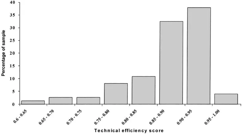
4.2. Technical efficiencies
Fig. 1 shows the frequency distribution of production-unit-specific technical efficiency, averaged over the period for which each farm appears in the sample. Predicted technical efficiencies range from a minimum of 49.51% to a maximum of 98.01%, the mean value being 87.01% with a standard deviation of 10.52%. More than 74% of the sampled farms have mean efficiency scores that are 85% or greater.
5 Ifγ=0 is involved in the null hypothesis (H
0), then the
like-lihood ratio statistic has asymptotically a mixed chi-square distri-bution, if H0 is true (Coelli, 1995), the critical value for this test
is taken from Kodde and Palm (1986) (p. 1246; Table 1).
6 Elasticities are calculated at the mean values of the input
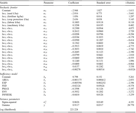
Table 5
Maximum-likelihood estimates for the parameters of the stochastic frontier and inefficiency effects model
Variable Parameter Coefficient Standard error t-Statistic
Stochastic frontier
Constant α0 −2.944 1.827 −1.611
ln x1(seed £/ha) α1 −2.816 0.773 −3.641
ln x2(fertiliser kg/ha) α2 1.056 0.814 1.297
ln x3(crop protection £/ha) α3 2.636 0.838 3.145
ln x4(labour h/ha) α4 0.1003 0.9118 0.110
ln x5(machinery h/ha) α5 0.3298 0.8195 0.402
ln x1×ln x1 α11 0.2300 0.0564 4.075
ln x1×ln x2 α12 0.2612 0.0960 2.720
ln x1×ln x3 α13 −0.0208 0.0706 −0.294
ln x1×ln x4 α14 −0.0184 0.1033 −0.178
ln x1×ln x5 α15 −0.0500 0.1207 −0.414
ln x2×ln x2 α22 0.1562 0.0602 2.594
ln x2×ln x3 α23 −0.3913 0.0819 −4.775
ln x2×ln x4 α24 −0.3033 0.0810 −3.742
ln x2×ln x5 α25 −0.2685 0.1123 −2.390
ln x3×ln x3 α33 −0.0799 0.0441 −1.810
ln x3×ln x4 α34 −0.0460 0.0829 −0.555
ln x3×ln x5 α35 0.1240 0.1131 1.096
ln x4×ln x4 α44 −0.0400 0.0463 −0.864
ln x4×ln x5 α45 0.4137 0.1242 3.330
ln x5×ln x5 α55 −0.00278 0.08514 −0.0326
Inefficiency model
Constant δ0 0.798 0.152 5.261
AREA δ1 −0.001175 0.000412 −2.853
EXP δ2 −0.005394 0.002252 −2.396
FED δ3 −0.02124 0.05624 −0.378
PMAX δ4 −0.3598 0.1126 −3.197
ENV δ5 −0.3932 0.1202 −3.272
INFSEEK δ6 −0.0410 0.0126 −3.259
Variance parameters
Sigma-squared σ2
s 0.0626 0.0149 4.191
Gamma γ 0.9117 0.0317 28.770
Log (likelihood) 221.224
5. Technical efficiency and managerial capacity
The results detailed in Section 4 show that the ma-jority of cereal farmers in this sample are operating relatively close to the fully efficient frontier. This is an unsurprising conclusion given that the summary statistics for the sample show that there is little varia-tion in yields and input applicavaria-tion rates. Despite this fact parameter estimates for the stochastic frontier and technical inefficiency effects model show that system-atic technical inefficiency effects exist and that these
are, in part, explained by the variables included in the model.
Fig. 1. Frequency distribution of predicted technical efficiencies.
and Coelli (1993) show that for the i-th firm in the t-th time period, technical efficiency is predicted using the conditional expectation
TEit=E[exp(−uit)|Eit=eit]
=exp(−µ∗+12σ∗2)
8[(µ
∗/σ∗)−σ∗]
8(µ∗/σ∗)
(5)
where
µ∗=(1−γ )zitδ−γ eit, σ∗2=γ (1−γ )σs2, eit=vit−uit
and 8 represents the distribution function of the standard normal random variable. Table 6 presents the results of differentiating Eq. (5) with respect to
Table 6
Marginal effects of inefficiency effects model variables Variable Coefficient Standard error t-Statistic
AREA 0.0000563 0.0000111 5.080
EXP 0.0002586 0.0000996 2.596
FED 0.00102 0.00270 0.377
PMAX 0.0173 0.0041 4.194
ENV 0.0188 0.00363 5.188
INFSEEK 0.00196 0.000477 4.122
each of the inefficiency effects variables (evaluated at their mean values or with a value of one for dummy variables and where the residuals, eit, are calculated at the mean values of the dependent and independent variables in the stochastic frontier function).
Table 6 shows that all these variables have a positive effect on levels of efficiency and that all, apart from the further education variable (FED), have a statisti-cally significant effect. Note that for those variables constructed as dummy variables (FED, PMAX and ENV), the coefficient estimated represents a one-off shift in efficiency rather than a true marginal effect.
farmers who rank maintaining the environment as an important objective. One possible explanation is that farmers who are environmentally aware, practice a more efficient use of inputs than those who are less environmentally aware.
The model also shows that managers with more experience and those with some form of further edu-cation are likely to be less inefficient than those man-agers with fewer years of experience and lower levels of education, although the estimated coefficient for the latter is statistically insignificant, and the effect in both cases is very small. The coefficient estimate associated with the AREA variable is also very small, although it is highly significant statistically and reinforces the findings of other UK specific studies (Dawson, 1985; Wilson et al., 1998) that technical inefficiency in-creases as farm size dein-creases. Given that the constant returns to scale model specification employed here, this is an interesting result, and may arise from the ability of larger farms to negotiate bulk buy discounts for the two inputs which are defined in cost terms (seeds and crop protection) which would then be re-flected in lower costs per ha than those for smaller farms.
6. Summary
Technical inefficiency in wheat yields in eastern England has been estimated and the variation in technical inefficiency explained using variables repre-senting a number of managerial biographical details, managerial drives and motivations and practices and procedures with respect to business planning. The results indicate that the majority of wheat farmers in eastern England operate close to maximum tech-nically feasible yield levels and that there is limited potential to improve technical efficiency.
Variables constructed to represent managerial busi-ness objective, profit maximisation and concern for maintaining the environment, are shown to have a significant and positive effect on levels of techni-cal efficiency. Moreover, increasing farm size and seeking information are also associated with higher levels of efficiency. The information-seeking variable was included in this research to examine the influ-ence of aspects of the managerial decision-making process. Our findings indicate that aspects of the
decision-making process do influence technical effi-ciency. This reinforces the suggestion of Rougoor et al. (1998) that further studies should include more infor-mation on aspects of the managerial decision-making process if they are to successfully measure farmers’ management capacity.
The results presented both reinforce findings from previous studies that examine the issue of technical efficiency and also highlight some of the factors that affect technical efficiency. Perhaps of most contem-porary interest is that those farmers who consider maintaining the environment as an important objec-tive achieve higher levels of technical efficiency. The results of this study therefore suggest that practices and business objectives that seek to maintain the en-vironment may, indirectly, lead to an improvement in technical efficiency.
Acknowledgements
The financial assistance of the Home-Grown Cereals Authority is gratefully acknowledged. We also wish to thank two anonymous referees for their constructive comments.
References
Aigner, D., Lovell, C.A.K., Schmidt, P., 1977. Formulation and estimation of stochastic frontier production function models. J. Econometrics 6, 21–37.
Asby, C., 1998. Economics of wheat and barley production in Great Britain. Special Studies in Agricultural Economics, Report No. 37, Agricultural Economic Unit, Department of Land Economy, University of Cambridge, UK.
Battese, G.E., Broca, S.S., 1997. Functional forms of stochastic frontier production functions and models for technical inefficiency effects: a comparative study for wheat farmers in Pakistan. J. Productivity Anal. 8, 395–414.
Battese, G.E., Coelli, T.J., 1988. Prediction of firm-level technical efficiencies with a generalized frontier production function and panel data. J. Econometrics 38, 387–399.
Battese, G.E., Coelli, T.J., 1993. A stochastic frontier production function incorporating a model for technical inefficiency effects. Working Papers in Econometrics and Statistics No. 69, Department of Econometrics, University of New England, Armidale.
Battese, G.E., Malik, S.J., Gill, M.A., 1996. An investigation of technical inefficiencies of production of wheat farmers in four districts of Pakistan. J. Agric. Econ. 47 (1), 37–49.
Coelli, T.J., 1995. Estimators and hypothesis tests for a stochastic frontier function: a Monte Carlo analysis. J. Productivity Anal. 6, 247–268.
Coelli, T.J., 1996. A guide to FRONTIER Version 4.1: a computer program for stochastic frontier production and cost function estimation. CEPA Working Paper 96/07, Centre for Efficiency and Productivity Analysis, University of New England, Armidale.
Davidson, D., Asby, C., 1995. UK Cereals, 1993/94: the impact of the CAP reform on production economics and marketing. Special Studies in Agricultural Economics, Report No. 28, Agricultural Economic Unit, Department of Land Economy, University of Cambridge, UK.
Dawson, P.J., 1985. Measuring technical efficiency from production functions: some further estimates. J. Agric. Econ. 36, 31–40. Greene, W.H., 1997. Frontier production functions. In: Pesaran,
M.H., Schmidt, P. (Eds.), Handbook of Applied Econometrics, Vol. II: Microeconomics. Blackwell Scientific Publications, Oxford (Chapter 3).
Huang, C.J., Liu, J.-T., 1994. Estimation of a non-neutral stochastic frontier production function. J. Productivity Anal. 5, 171–180. Jondrow, J., Lovell, C.A.K., Materov, I.S., Schmidt, P., Econo-metrics, J., 1982. On the estimation of the technical inefficiency
in the stochastic production function model. J. Econometrics 19, 233–281.
Judge, G.C., Griffiths, W.E., Hill, R.C., Lütkepohl, H., Lee, T.-C., 1985. The Theory and Practice of Econometrics, 2nd Edition. Wiley, New York.
Kay, R.D., Edwards, W.M., 1994. Farm Management. McGraw-Hill, New York.
Kodde, D.A., Palm, F.C., 1986. Wald criteria for jointly testing equ-ality and inequequ-ality restrictions. Econometrica 54, 1243–1248. Kumbhakar, S.C., Ghosh, S., McGuckin, J.T., 1991. A generalized production frontier approach for estimating the determinants of inefficiency in US dairy farms. J. Bus. Econ. Statist. 9, 279–286. MAFF, 1997. June census data 1996. Internal Communication,
Ministry of Agriculture Fisheries and Food, London. Meeusen, W., van den Broeck, J., 1977. Efficiency estimation from
Cobb–Douglas production function with composed error. Int. Econ. Rev. 18, 435–444.
Reifschneider, D., Stevenson, R., 1991. Systematic departures from the frontier: a framework for the analysis of firm inefficiency. Int. Econ. Rev. 32, 715–723.
Rougoor, C.W., Trip, G., Huirne, R.B.M., Renkema, J.A., 1998. How to define and study farmers’ management capacity: theory and use in agricultural economics. Agric. Econ. 18, 261–272. Wilson, P., Hadley, D., Ramsden, S., Kaltsas, I., 1998. Measuring