On the realistic stochastic model of GPS observables: Implementation and Performance
F. Zangeneh-Nejad a,*, A. R. Amiri-Simkooei b, M. A. Sharifi a , J. Asgari b
a School of Surveying and Geosptial Engineering, Research Institute of Geoinformation Technology (RIGT), College of Engineering, University of Tehran, Iran- (f.zangenehnejad, [email protected])
c Department of Geomatics Engineering, Faculty of Engineering, University of Isfahan, 81746-73441 Isfahan, Iran- (amiri, [email protected])
KEY WORDS: GPS stochastic model, Least-squares variance component estimation (LS-VCE), noise assessment, integer
ambiguity resolution (IAR), Success rate, GPS observables.
ABSTRACT:
High-precision GPS positioning requires a realistic stochastic model of observables. A realistic GPS stochastic model of observables should take into account different variances for different observation types, correlations among different observables, the satellite elevation dependence of observables precision, and the temporal correlation of observables. Least-squares variance component estimation (LS-VCE) is applied to GPS observables using the geometry-based observation model (GBOM). To model the satellite elevation dependent of GPS observables precision, an exponential model depending on the elevation angles of the satellites are also employed. Temporal correlation of the GPS observables is modelled by using a first-order autoregressive noise model. An important step in the high-precision GPS positioning is double difference integer ambiguity resolution (IAR). The fraction or percentage of success among a number of integer ambiguity fixing is called the success rate. A realistic estimation of the GNSS observables covariance matrix plays an important role in the IAR. We consider the ambiguity resolution success rate for two cases, namely a nominal and a realistic stochastic model of the GPS observables using two GPS data sets collected by the Trimble R8 receiver. The results confirm that applying a more realistic stochastic model can significantly improve the IAR success rate on individual frequencies, either on L1 or on L2. An improvement of 20% was achieved to the empirical success rate results. The results also indicate that introducing the realistic stochastic model leads to a larger standard deviation for the baseline components by a factor of about 2.6 on the data sets considered.
* Corresponding author
1. INTRODCTION
GPS data processing is usually performed by the least squares adjustment method for which both the functional and stochastic models must be correctly specified. The functional model, describing the mathematical relation between the observations and the unknown parameters, is usually well known either in the relative positioning or in the single/precise point positioning (Seeber, 2003; Hofmann-Wellenhof et al., 2008; Leick, 2004; Teunissen and Kleusberg, 1998; Rizos, 1997). However, the stochastic model, expressing the statistical characteristics of the GPS observations by means of a covariance matrix, is still a challenging problem. Misspecification in the stochastic model leads to unreliable and suboptimal estimates. The realistic stochastic model should thus be utilized aiming at obtaining reliable least squares estimates.
There are a few common stochastic models for GPS observables: (1) Equal-weight stochastic model in which identical variances for each measurement type are chosen (i.e. the same variance for the code and the same variance for the phase observations). This structure ignores the correlations among different observables, (2) Satellite elevation-angle dependent model in which the observations weighting procedure is performed using trigonometric or exponential functions. The observations at lower elevation angles have larger variances than those at higher elevation angles, (3) Signal-to-noise ratio (SNR) based model in which the
observations weighting procedure depends on SNR values, a quality indicator for the GPS observations. These models are in fact simple and rudimentary stochastic models. Satirapod and Wang (2000) found that in some cases both the use of SNR and satellite elevation angle information failed to reflect the reality of data quality. Therefore, it still remains necessary to investigate rigorous methods for constructing a more reliable covariance matrix of the GPS observables. An appropriate stochastic model for GPS observables may include different variances for each observation type, the correlation among different observables, the satellite elevation dependence of observables precision, and the possible temporal correlation of the GPS observables (Amiri-Simkooei et al., 2009, 2013, 2015). Therefore, we first define a general form of the covariance matrix of the GPS observables, which includes the above-mentioned variance and covariance components into the stochastic model. This general form of the covariance matrix is expressed as an unknown linear combination of known cofactor matrices. The estimation of the unknown (co)variance parameters is referred to as variance component estimation (VCE).
There are many different methods for VCE among which we make use of the least-squares variance component estimation (LS-VCE), in a straightforward manner, to assess the noise characteristics of the GPS observables. LS-VCE was originally developed by Teunissen (1988). Further elaboration and development of the LS-VCE are provided by Teunissen and
Amiri-Simkooei (2008) and Amiri-Simkooei (2007). The geometry-based observation model (GBOM), employed as the functional model, is the widely used mathematical model for high precision GPS positioning from code and phase observations using a relative GPS receiver setup (Odijk, 2008).
An important step in the high-precision GPS positioning is double difference (DD) integer ambiguity resolution (IAR). The fraction or percentage of success among a number of integer ambiguity fixing is called the success rate. A realistic estimation of the GNSS observables covariance matrix plays an important role in the IAR. When compared to a realistic stochastic model, a simple stochastic model results in poorer precision of the estimated parameters and hence a lower integer ambiguity success rate. In this paper, the reliability of the resolved ambiguities is investigated through the computation of the IAR success rate for two cases, namely a nominal and a realistic stochastic model of the GPS observables. For the nominal case, the same standard deviations for the phase observables on L1
respectively. This structure ignores the correlation among different observables, the satellite elevation dependence of observables precision, and the possible temporal correlation of the GPS observables.
The baseline components uncertainties expressed by the estimated covariance matrix of the unknowns depend on the choice made for the weight matrix of the observables. We thus assess the effect of the stochastic model on the efficiency of the estimated baseline uncertainties. To this end, the baseline uncertainties are also computed for two cases, nominal and a realistic stochastic model of the GPS observables.
This paper is organized as follows. Section 2 provides a brief review on a few theoretical concepts followed in this research. This section reviews the functional part of the GPS GBOM, a realistic stochastic model of GPS observables. Section 3 presents the theory of the LS-VCE method and its application to determine an appropriate stochastic model. In section 4, to investigate the performance of the realistic stochastic model obtained by the LS-VCE approach, two GPS baseline data sets of short baselines are employed. The reliability of the resolved ambiguities is then investigated through the computation of the IAR success rate for two cases, namely a nominal and a realistic stochastic model of the GPS observables. We also assess the effect of the stochastic model on a realistic standard deviation for the baseline components. We further highlight the effect of an optimal stochastic model in other fields of GPS applications such as the precise point positioning method. Finally, we make conclusions in section 6.
2. GPS GEOMETRY-BASED OBSERVATION MODEL
(GBOM)
2.1 Functional model
Consider two receivers r and j simultaneously track the same satellites s and k. The functional part of GBOM is based on the DD GPS observables. Ignoring the DD atmospheric delays, which is a valid assumption for zero and very short baselines, the observation equation for the DD GPS pseudorange (code) and carrier phase observations are respectively defined as (Teunissen and Kleusberg, 1998) L1 or L2 frequency,
denotes the DD receiver-satellite range,e
indicates the pseudorange measurement errors on the L1 or L2 frequency andt
i refers to the measurement time instant. InEq. (2),
indicates the DD carrier phase observation on the L1or L2 frequency,
is the corresponding wavelength, a denotes the DD integer ambiguities on L1 or L2, and
is the phase measurement errors on L1 or L2.The DD pseudorange and carrier-phase observation equations on the L1 or L2 frequency can be written in the following
relating to two satellites which were observed by two receivers. In Eq. (3), E stands for the mathematical expectation operator. The expectation of pseudorange and carrier-phase measurement errors is assumed to be zero. In Eq. (3), the design matrix A is unknown baseline components between the reference and rover
receivers, which is defined as
T rj rj rj g X Y Z .
2.2 A Realistic Stochastic Model
A realistic stochastic model for DD GPS observables is of the form (Amiri-Simkooei et al., 2009, 2013, 2015)
D
y C T E
Q (5)
where
indicates the Kronecker product of two matrices. For four observation types C includes 10 unknown variance and variances and the covariance between the GPS observables, respectively.Also, a Toeplitz matrix
T represents temporal correlation of the GPS observables. It is a K
K matrix, where Kdenotes the number of the observation epochs.T
may consists of Knumber of unknown parameters as follows
( 0 ) (1) ( 1) the number of satellites. The satellite number [1] is assumed as
the reference satellite. E is of the form
The stochastic model presented in Eq. (5) considers all items of a realistic covariance matrix of GPS observables pointed out in the introduction. In this paper, we estimate the unknown (co)variance components using LS-VCE which is briefly presented in the next section.
3. STOCHASTIC MODEL ESTIMATION
3.1 Least-Squares Variance Component Estimation
(LS-VCE)
The LS-VCE was originally developed by Teunissen (1988). Further elaboration and development of the method is provided by Teunissen and Amiri-Simkooei (2008) and Amiri-Simkooei (2007).
Assume the linear model of observation equations as
1
where D denotes the mathematical dispersion operator, y is the observation vector of order m, x is the n-vector of unknown parameters, A is the m n
design matrix describing the functional relation between the observations vector and theunknown parameters and
k,
k
1,...,
p are the unknown (co)variance components. Also, Qy is the covariance matrix ofthe observables expressed as an unknown linear combination of
known cofactor matrices (Qk
,
k
1,...,
p).Based on Eq. (9), the covariance matrix of the observables is partly unknown as it is expressed as an unknown linear combination of known cofactor matrices. To estimate the unknown (co)variance components, different VCE methods have been invented. Among them the LS-VCE method is employed in the present contribution.
The unknown (co)variance components can be estimated using
LS-VCE as
ˆ
N l1 , where the p
p matrix N and thep-vector l are respectively obtained as projector, and
tr
denotes the trace of a matrix.To compute the matrix N, the vector l and the residuals vector e
ˆ
the covariance matrix of the observables is required. LS-VCE is thus an iterative method that needs the approximate values of the (co)variance components. The iteration proceeduntil the converge criterion of
ˆj ˆj1
is met, i.e., the difference of two consecutive solutions is less than the tolerance
. The covariance matrix of the estimated (co)variance components can automatically be obtained as Qˆ N1.When the number of observations is large, we can divide the entire observations into a few (r) groups. One can show that the
unknown (co)variance parameters
(
k;
k
1 : )
p
can bekth co(variance) components of the ith group (Amiri-Simkooei et method may be applied to GPS GBOM as the functional model in three ways, namely Float ambiguities, Fixed ambiguities and Fixed ambiguities and fixed baseline (Amiri-Simkooei et al. 2013, 2015). In this paper, we carried out the Fixed ambiguities method. After fixing the DD integer ambiguities via the least-squares ambiguity decorrelation adjustment (LAMBDA) method (Teunissen, 1993, 1995) or the lattice theory (Jazaeri et al., 2012), the fixed DD integer ambiguities were moved to the left hand side of Eq. (3). In this case, A simplifies
to
A
[
G G G G
T T T T].
TEquation (5) presents a realistic stochastic model of GPS observables. Estimation of the (co)variance components of this model may be performed in there steps (1) Estimation of the Amiri-Simkooei et al. (2009, 2013, 2015).
3.2.1 Estimation of (co)variance components of
C: In thefirst stage, the (co)variance components
C including the different variances of observation types and the possible correlation among the GPS observables are estimated. For this purpose, the temporal correlation and the satellites elevation dependence of GPS observables precision are ignored. On themeaning that all satellites with different elevation angles have
equal variance factors (i.e.,
[1]2
[ 2 ]2
[ ]2k ).By using the structure introduced in Eq. (15) for
E andT
I
K
, the (co)variance components ofC
can be estimated by LS-VCE. The approximate values for the covariance components was assumed to be zero, un-correlated observables, and the approximate values for the standard deviation of GPS code (C1 and P2) and phase observations (L1 and L2) were taken as 30 cm and 3 mm, respectively. Also, the tolerance for the convergence of the LS-VCE solution is set to = 10-6.3.2.2 Estimation of components of
E: After estimating the(co)variance components of
C, we may consider the satellites elevation dependence of GPS observables precision byestimating the components of
E using LS-VCE. To this end, matrix
C, which is already estimated, is introduced into the stochastic model of Eq. (5). The temporal correlation is stillassumed to be absent at this stage, i.e.,
TI
K. The components of
E can then be estimated using LS-VCE. Also, the approximate values for the variance factors of
E are the satellites elevation, an exponential elevation-dependent model may also be used. This model is similar to the Euler and Goad elevation-dependent model (Euler and Goad, 1991), andelevation angle of the satellites and
0 is an unknown reference elevation angle. The unknown parameters of the nonlinear model given in (16) can be obtained by a nonlinear least squaresfit to the estimated variance components of
E using LS-VCE. Therefore, the exponential elevation-dependent model was implemented to express the dependence of the GPS observable precision on the satellite elevation angle (Amiri-Simkooei et al., 2015).3.2.3 Estimation of components of
T: In the last step,time correlation of the GPS observables is investigated. At this
stage, the components of using the empirical autocovariance function (ACF), which is shown to be a by product of the LS-VCE method, if the weight matrix is chosen as the identity matrix. The unbiased sample autocovariance function of a zero-mean stationary time-series can be obtained as (Amiri-Simkooei 2007, p. 42)
1
where
is the time lag (the time interval between two samples)in seconds,
is the covariance among the observables withlag
and K is the number of epochs. The coefficient at lag0
equals the diagonal elements (variance factors) of
T.As a predefined model, the temporal correlation of the GPS observables is approximated by an exponential auto covariance function (first-order auto regressive, AR(1)) as
2 can be obtained by a nonlinear least squares fit to the estimated
ˆ
obtained by Eq. (17). Therefore, the exponential auto covariance function was implemented to express the temporal correlation of the GPS observables.4. NUMERICAL RESULTS AND DISCUSSIONS
To investigate the effect of the realistic stochastic model of the GPS observables on the IAR success rate and on the estimated baseline uncertainties, two real GPS data sets collected by a geodetic GPS receiver, namely Trimble R8, are employed. The receiver used is a geodetic dual frequency receiver which provides the code and phase observations on both the L1 and L2 frequencies (namely, C1-P2-L1-L2). The first GPS data experiment was collected on November 28, 2010 with one second interval over a short baseline of 2.5892 m from 13:11:19 to 13:15:28 UTC consisting of 250 epochs. The second data set was also measured over a short baseline of 20.526 m with one second interval on November 28th, 2010, from 13:17:18 to 13:21:27 UTC consisting of 200 epochs.
This geodetic GPS receiver has been recently used in Amiri-Simkooei et al. (2015) for two different GPS data sets. We now use other datasets using the same receiver under a different situation, for example different days and different satellite configuration. However, we use the standard deviation of the phase and code observations as well as the correlation coefficient among different observations as those estimated by Amiri-Simkooei et al. (2015). correlation coefficients between the GPS observables. The results indicate a significant correlation between observations. A positive correlation of 0.42 is observed between the phase observations on L1 and L2 for Trimble R8, which is considered to be significant (see Amiri-Simkooei et al., 2013). The
estimated values of the parameters given in (16) are a1
0.26
,2 18.90
a and the reference angle is estimated as
0 7.6 , for the Trimble R8 receiver.Table 1. Estimated covariance
ˆi j, (mm2) and correlationcoefficient
ˆi j, among different observations for Trimble R8Between 2
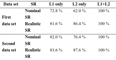
After introducing the estimated components of
C three following cases: Case (1): L1 only; Case (2): L2 only and
Case (3): L1 + L2. The empirical success rate computed for
three cases are given in Table (2). The results indicate that
applying the estimated components of
C and
E to the mathematical model of the GPS baselines can significantly improve the success rate; an improvement of 20% is clear when using only L1 or L2.Table 2. Estimated empirical success rate (SR) for each of GPS
data sets in three cases. also showed that applying a more realistic stochastic model can significantly improve the IAR success rate on individual frequencies, either on L1 or on L2. This work can be considered as a follow-up to the work carried out by Amiri-Simkooei et al. (2015) in which some supplementary results, for example considering the effect of introducing the realistic stochastic model on the estimation of the two baseline components uncertainties, are also presented in this contribution.
We now aim to consider the effect of introducing the realistic stochastic model on the estimation of the baseline components uncertainties. The baseline uncertainties can be regarded as the square root of the diagonal components of the unknowns
covariance matrix approximated by Qxˆ (A Q AT y1 )1 in which
y
Q can be considered in three different cases:
Case I: Nominal stochastic model of the GPS
observables,
Case II: A realistic stochastic model of the GPS
observables by introducing the
C and
E matrices estimated by the LS-VCE method, Case III: Considers the
C
andE
as estimated in Case II. In addition, the realistic stochastic model of the GPS observables considers time correlation of GPS observables based on the empirical ACF and fitting an exponential auto covariance function to the ACF.Table (3) provides the estimated baseline uncertainties in the three cases for each of the GPS data sets. The results indicate that the estimated baseline uncertainties in the case of the nominal stochastic model lead to the optimistic uncertainties of the estimated baseline components when compared to a realistic stochastic model (cases II and III). In other words, introducing the realistic stochastic model results in a larger standard deviation for the baseline components by a factor of about 2.6 on the data sets considered.
Table 3. Estimated baseline uncertainties in three cases for two
data sets: Case I: Nominal, Case II: considering
C and
E and Case III: considering
C ,
E and
T.Data set Case
X
(mm)
Y (mm)
Z (mm)First
data set
I 0.27 0.34 0.36
II 0.35 0.50 0.43
III 0.66 0.85 0.90
Second
data set
I 0.27 0.36 0.38
II 0.34 0.49 0.45
III 0.76 1.03 1.09
In this paper, we investigated the effect of an optimal stochastic model in the case of relative positioning. The choice of a realistic stochastic model of the GPS observables is also important in other fields of GPS applications such as the precise point positioning (PPP) technique.
5. CONCLUSIONS
A realistic stochastic model for the GPS observables should include a few important issues like different variances for each GPS observation type, the correlation between different observations, the satellite elevation dependence of the GPS observables weights, and the temporal correlation of the GPS observables. The use of a proper (correct) stochastic model of the GPS observables leads to the best linear unbiased estimators (BLUE) in the high precision GNSS positioning. The LS-VCE method was applied to GPS observables using the GBOM as the functional model.
The impact of a realistic GPS stochastic model on IAR success rate was discussed using two GPS short baseline data sets. The empirical success rate was computed for two cases: (1) using the nominal covariance matrix, and (2) using the estimated covariance matrix by LS-VCE. For the latter case, the success rate is determined by taking into consideration the variances of the GPS observables, the covariance/correlations of GPS observables, and the satellites elevation dependence of the GPS observable precision. The results showed that applying a more realistic stochastic model can significantly improve the IAR success rate on individual frequencies, either on L1 or on L2. An improvement of 20% was achieved to the success rate results. This idea can thus be implemented in attitude determination using single-frequency single-epoch of GPS
observations in order to improve and/or speed up the ambiguity fixing procedure.
Finally, the effect of the realistic stochastic model on the estimated baseline uncertainties was investigated. The results indicated that introducing the realistic stochastic model leads to a larger standard deviation for the baseline components by a factor of about 2.6 on the data sets considered.
ACKNOWLEDGEMENTS
We would like to acknowledge Dr. Shahram Jazaeri for providing us with the GPS data sets we used in this paper.
REFERENCES
Amiri-Simkooei, AR., 2007. Least-squares variance component estimation: Theory and GPS applications. Ph.D. thesis, Delft Univ. of Technology, Delft, The Netherlands.
Amiri-Simkooei, AR., Teunissen, PJG., Tiberius, CCJM., 2009. Application of least-squares varinace component estimation to GPS observables. J Surv Eng., 135(4):149-160.
Amiri-Simkooei, AR., Zangeneh-Nejad, F., Asgari, J., 2013. Least-squares variance component estimation applied to GPS geometry-based observation model. J Surv Eng., 139(4):176-187.
Amiri-Simkooei, AR., Zangeneh-Nejad, F., Jazaeri, S., Asgari, J., 2015. Role of stochastic model on GPS integer ambiguity resolution success rate, GPS Solutions, DOI 10.1007/s10291-015-0445-5.
Euler, HJ., Goad, C., 1991. On optimal filtering of GPS dual frequency observations without using orbit information. Bull. Geod, 65: 130–143.
Hofmann-Wellenhof, B., Lichtenegger, H., Wasle, E., 2008. GNSS Global Navigation Satellite Systems – GPS, GLONASS, Galileo & more. Springer, Wien New York.
Jazaeri, S., Amiri-Simkooei, AR., Sharifi, MA., 2012. Fast integer least-squares estimation for GNSS high-dimensional ambiguity resolution using lattice theory. J Geodesy, 86(2):123–136.
Leick, A., 2004. GPS Satellite Surveying. 3rd edition, John Wiley, New York.
Odijk, D., 2008. GNSS Solutions: What does geometry-based and geometry-free mean in the context of GNSS? Inside GNSS, 3(2), 22–24.
Rizos, C., 1997. Principles and practice of GPS surveying. Monograph 17, School of Geomatic Engineering, The University of New South Walse, Sydney.
Satirapod, C., Wang, J., 2000. Comparing the Quality Indicators of GPS Carrier Phase Observations, Geomatics Research Australasia.
Seeber, G., 2003. Satellite Geodesy. De Gruyter, Berlin.
Teunissen, PJG., 1993. Least squares estimation of the integer GPS ambiguities. Proc., IAG General Meeting, Series No. 6, Delft Geodetic Computing Centre.
Teunissen, PJG., 1995. The least-squares ambiguity decorrelation adjustment: A method for fast GPS integer ambiguity estimation. J Geodesy, 70(1–2):65–83.
Teunissen, PJG., 1988. Towards a least-squares framework for adjusting and testing of both functional and stochastic model. Internal research memo, Geodetic Computing Centre, Delft. A reprint of original 1988 report is also available in 2004, No. 26
Teunissen, PJG., Kleusberg, A., 1998. Section 7: Quality control and GPS. GPS for Geodesy, PJG, Teunissen and A, Kleusberg, eds., Springer, Berlin.
Teunissen, PJG., Amiri-Simkooei, AR., 2008. Least-squares variance component estimation. J. Geodesy, 82(2), 65–82.