Forward-futures price differences in the UK commercial property market Arbitrage and marking-to-model explanations.

(1)

Forward

–

_{futures price differences in the UK commercial property}

market: Arbitrage and marking-to-model explanations

Silvia Stanescu, Radu Tunaru

⁎

_{, Made Reina Candradewi}

Kent Business School, University of Kent, CT2 7PE, United Kingdom

a b s t r a c t

a r t i c l e

i n f o

Article history: Received 9 January 2014

Received in revised form 27 May 2014 Accepted 30 May 2014

Available online 12 June 2014 JEL classiﬁcation:

C12 C33 G13 G19 Keywords:

Total return swaps and futures Panel data

Mean-reversion Markov Chain Monte Carlo

In this paper the differences between forward and futures prices for the UK commercial property market are analyzed, using both time series and panel data. Aﬁrst battery of tests establishes that the observed differences are statistically signiﬁcant over the study period. Further analysis considers the modeling of this difference using mean-reverting models. The proposed models are then estimated with a number of alternative estimation methods and second stage statistical tests are implemented in order to decide which model and estimation method best represent the data.

1. Introduction

The difference between forward and futures prices has been given considerable attention in thefinance literature, both from a theoretical as well as from an empirical perspective, and for various underlying assets. On the theoretical side,Cox, Ingersoll, and Ross (1981)(CIR) obtained a relationship between forward and futures prices based solely on no-arbitrage arguments.1_{A series of papers subsequently tested} em-pirically the CIR result(s).Cornell and Reinganum (1981)investigated whether the difference between forward and futures prices in the for-eign exchange market is different from zero. For several maturities and currencies, they found that the average forward–futures difference is not statistically different from zero. In addition, they suggested that earlier studies identifying significant forward–futures differences for the Treasury bill markets ought to seek explanations elsewhere than in the CIR framework, since the corresponding covariance terms for this market were even smaller.French (1983)reported significant

differences between forward and futures prices for copper and silver. Moreover, he conducted a series of empirical tests of the CIR theoretical framework and concluded that his results are in partial agreement with this theory.Park and Chen (1985)also investigated the forward–futures differences for a number of foreign currencies and commodities and they pointed out to signiﬁcant differences for most of the commodities that they analyzed, but not for the foreign currencies. Also, their empir-ical tests conﬁrmed that the majority of the average forward–futures price differences are in accordance with the CIR result.

Kane (1980)tried to explain the differences between futures and forward prices based on market imperfections such as asymmetric taxes and contract performance guarantees.Levy (1989) strongly argued that the difference between forward and futures prices arises from the marked-to-market process of the futures contract. Meulbroek (1992)investigated further the relationship between for-ward and futures prices on the Eurodollar market and suggested that the marked-to-market effect has a large inﬂuence. However,Grinblatt and Jegadeesh (1996) advocated that the difference between the futures and forward Eurodollar rates due to marking-to-market is small.Alles and Peace (2001)concluded that the 90-day Australia futures prices and the implied forwards are not fully supported by the CIR model. Recently,Wimschulte (2010)showed that there is no signif-icant statistical or economical evidence for price differences between electricity futures and forward contracts.

⁎ Corresponding author. Tel.: +44 1227 824608. E-mail address:R.Tunaru@kent.ac.uk(R. Tunaru).

1

Other early studies that considered the relationship between forward and futures prices in a perfect market without taxes and transaction costs areMargrabe (1978), Jarrow and Oldﬁeld (1981)andRichard and Sundaresan (1981).

Contents lists available atScienceDirect

(2)

The relationship between forward and futures prices as developed under the CIR framework makes the tacit assumption that futures are infinitely divisible.Levy (1989)starts with the same set of assumptions underpinning the CIR model except one. When considering interest rates, he advocates that, if only the next day's interest rate were deter-ministic, a perfect hedge ratio using fractional futures positions can be constructed to replicate the forward. Thus, forLevy (1989)it is only the interest rate for the next day that is important and not the entire time path of the stochastic rates. Consequently, forLevy (1989), the for-ward pricesshould be equalto futures prices and any empiricalfindings regarding actual price differentials are non-systematic and they can have onlystatisticalexplanations. On the other hand,Morgan (1981) studied the forward–futures differential assuming that capital markets are efficient and concluded that forward and futures prices must be dif-ferent. His conclusion is mainly based on the fact that current futures price depends on the joint future evolution of stochastic interest rates and futures prices.Polakoff and Diz (1992)argued that due to the indi-visibility of the futures contracts,2_{the forward prices}_{should be different} from futures prices even when interest rates and futures prices exhibit zero local covariances. Moreover, they show that the autocorrelation in the time series of the forward–futures price differences should be expected. Hence, testing must take into consideration the presence of autocorrelation.Polakoff and Diz (1992)offered a theoretical explana-tion that unifies the contradictory theoretical views originated in how interest rates are negotiated in the model. Their main conclusion is that it is unnecessary for futures prices and interest rates to be correlat-ed in order to imply that forward prices should be different from futures prices.

From the review discussed above it appears that the empirical evidence is mixed and asset class specific. Property derivatives are an emerging asset class of considerable importance forfinancial systems. Case and Shiller (1989, 1990)found evidence of positive serial correla-tion as well as inertia in house prices and excess returns, implying that the U.S. market for single-family homes is inefficient. The use of deriva-tives for risk management in real estate markets has been discussed by Case, Shiller, and Weiss (1993),Case and Shiller (1996)andShiller and Weiss (1999) with respect to futures and options. Fisher (2005) discussed NCREIF-based swap products, whileShiller (2008)described the role played by the derivatives markets in general for home prices.

For real-estate there has been a perennial lack of developments of derivatives products that could have been used for hedging price risk. The only property derivatives traded more liquidly in the U.S. and the

U.K. are the total return swaps (TRSs), forwards and futures. In the U.K. commercial property sector for example, all three types of contract have the Investment Property Databank (IPD) index as the underlying. Since February 2009 the European Exchange (Eurex) has listed the UK property index futures. The most liquid derivatives markets on the IPD UK index are the TRS, which is an over-the-counter market, and the futures, both with at leastfive yearly market calendar December maturities. Any portfolio of TRS contracts can be decomposed into an equivalent portfolio of forward contracts. Hence, having data on TRS prices and futures prices opens the opportunity to compare, after somefinancial engineering, forward curves with futures curves on the IPD index. As remarked byPolakoff and Diz (1992)it is difficult to compare forward and futures prices on a daily basis when forwards are traded on a non-synchronous basis. By contrast, when forwards are derived on an implied basis from other instruments then matching the term-to-delivery is easy.

In this paper the forward–futures price differences are investigated for the UK commercial property market for allfive December market maturities. To our knowledge, this is thefirst study that considers the forward–futures price differences for this important asset class. The analysis of the difference is particularly important for two main reasons. Firstly, previous literature addressing the issue for different asset classes found that the empirical evidence was mixed and asset specific. There-fore, addressing the question for a new asset class is not an exercise of confirming previous results, but rather a new and important question in itself, especially since unexplained forward–futures differences can signal arbitrage opportunities. Secondly, intrinsic characteristics of real estate as an asset class make the contribution of this paper particularly relevant, since the underlying (a commercial real estate index in our case) is likely to be correlated with interest rates. According to the CIR result, this in turn should drive significant differences between forward and futures prices, but does this fully explain observed differences or can these occur, at least partially, due to arbitrage also? This is essential-ly what our paper aims to address. Furthermore, all previous studies relied exclusively on time series analysis, whereas in this paper we also conduct statistical tests for panel data as well as time series tests. To the authors' knowledge, this is thefirst study that considers panel data modeling in this context. Employing panel data has a series of advantages over basingfindings on time series alone.3For example, it increases statistical accuracy by increasing the number of degrees of freedom, which is particularly important for this application which benefits from having access to a unique OTC data set, with a relatively limited sample period, but with data available for a number of cross sec-tions. To sum up the contribution of the paper, we analyze the forward–

2

Although the vast majority of literature on futures is based on the assumption of inﬁ -nite divisibility,Polakoff (1991)discusses the important role played by the indivisibility of

futures contracts. 3

See, for exampleHsiao (2003)for a discussion of the advantages of using panel data.

(3)

futures difference for a new and particularly important asset class, employing a unique data set and providing panel test results, to our knowledge, for theﬁrst time in this stream of literature.

In addition, several models and estimation methods for the IPD index are investigated to try to determine which ones best capture the IPD forward–futures price difference. Empirical properties of real-estate indices suggest that the family of mean-reverting models presented inLo and Wang (1995)could be suitable for defining our modeling framework.Shiller and Weiss (1999)pointed out that the exact models advocated inLo and Wang (1995)may not be appropriate for real-estate derivatives since the underlying asset is not costlessly tradable, and they advocated using a lognormal model combined with an expected rate of return rather than a riskless rate. Later on,Fabozzi, Shiller, and Tunaru (2012)designed a way to merge the best of the two worlds by completing the market with the futures contracts that are used directly to calibrate the market price of risk for the real-estate index and hence, indirectlyfixing also the risk-neutral pricing measure which can be then applied for pricing other derivatives. There-fore, thefirst model we propose inSection 4below will be a slight modification of theLo and Wang (1995)trending OU process, where futures prices are used to calibrate the market price of risk, as pointed out inSection 4.3.

Real-estate prices exhibit serial correlation leading to a high degree of predictability, up to 50% R-squared for a short term horizon. More-over, it has been documented that returns on real-estate indices are positively autocorrelated over short horizons and negatively correlated over longer horizons, seeFabozzi et al. (2012).

The remainder of the paper is organized as follows:Section 2focuses on describing the data,Section 3contains the analysis that is real-estate model-free and the testing methodology covering panel data as well, Section 4contains the modeling approach taken for the commercial property index (including alternative estimation methods for the pro-posed models) and it also describes the second stage, model based tests.Section 5concludes.

2. Data description

For the empirical analysis of the differences between the forward and futures prices on the IPD4_{UK property index two types of tests} are performed. Firstly, it is investigated whether the observed difference between the forward and futures prices is statistically different from zero. Secondly, a number of established continuous time models com-bined with various methods of estimation are compared in order to

identify the model or models that are able to best capture this differ-ence. Using the previously defined notation, there are:n= 5 different maturities andN= 71 daily observations for each maturity. The data needed for this study contains IPD property futures prices, the IPD total return swap (TRS) rates, the IPD index, and also the GBP interest rates needed to calculate discount factors. Futures prices have been ob-tained from the European Exchange (Eurex5_{), the property TRS data} (thefixed rate) has been provided by Tradition Group, a major dealer on this market and the IPD index was sourced from the Investment Property Databank (IPD6_{). In addition, the UK's interest rates have} been downloaded from Datastream. Due to the limited availability of the property futures and TRS data, the sample period used is daily from 4 February 2009 until 7 July 2009. It generates 71 property futures daily curves and 71 sets of TRS rates with up tofive years maturity (the

ﬁrst maturity date is 31 December 2009, the second maturity date is 31 December 2010, the third maturity date is 31 December 2011, the fourth maturity date is 31 December 2012, and theﬁfth maturity date is 31 December 2013).

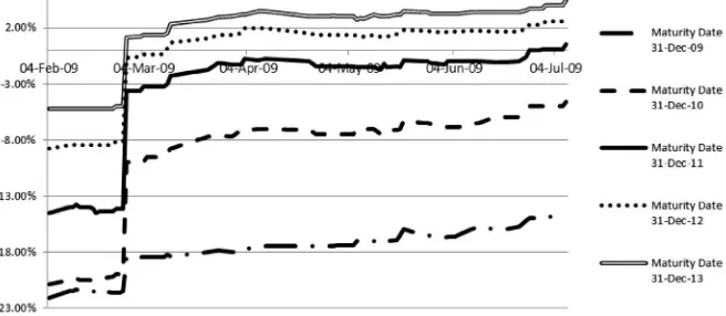
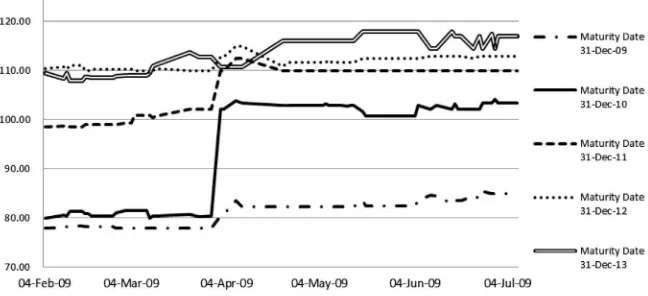
The evolution of the TRS series is depicted inFig. 1and one could see that, for our period of investigation, most of the IPD TRS rates are nega-tive for thefirst, second, and third maturity dates. We note that the total return swap rates are given as afixed rate and not as a spread over LIBOR.7_{A negative total return swap rate implies that the underlying} commercial property market will depreciate over the period to the ho-rizon indicated by the maturity of the contract. For the fourth andfifth maturity dates, the TRS rates are mostly positive. In addition, there is a dramatic increase of thefixed rate at the end of February 2009, possibly due to the rollover off the futures contracts in March combined with the publication of the IPD index for the year ending in December 2008. The property futures prices, quoted on a total return basis, are illustrated in Fig. 2. Futures prices are given on a total return basis so a futures price of 110 for December 2012 implies that the market expects a 10% appreci-ation of the commercial property in the UK at this horizon.

From the daily TRS prices for the marketﬁve yearly maturities one can reverse engineer the equivalent no-arbitrage forward prices for the same maturities. The equivalent fair property forward prices are de-rived daily from 4 February until 7 July 2009, with maturities matching the futures contracts maturities.

4

IPD stands for Investment Property Databank. A detailed description of the data is giv-en inSection 3.1below.

5

Seewww.eurexchange.comfor more information on Eurex. IPD UK futures contracts started on 4 February 2009.

6_See_www.ipd.com_{for more information on IPD.} 7

The TRS rate was initially equal to LIBOR plus a spread, but due to disagreements over what the spread should have been equal to, the property TRS swap rate is now equal to a ﬁxed rate, which is established upfront and can be negative.

(4)

Using data on theﬁxed rate of total return swap, UK interest rates and the monthly IPD all property total return index, the fair forward prices for property derivatives can be obtained. The following are the steps in constructing the fair prices of property forwards:

1. Calculate the adjusted discount factor.

adj discount factor¼discount factor ðT−tÞ intðT−tÞ þ1:

2. The gross mid TRS is obtained from:

gross mid TR¼sum of adj dfthe fixed rate of TRSðT;tÞ:

3. The projected calendar mid TR is calculated (in percentages):

projected calendar mid TR¼Δgross mid TRadj df

100 :

4. We can now obtain the projected index level as:

projected index level¼previous index level

ð1þprojected calendar midÞ:

5. Finally, the fair forward prices are generated (quoted in bp).

fair forward prices Tð ;tÞ ¼

projected index level Tð Þ

projected index level Tð −1Þ100:

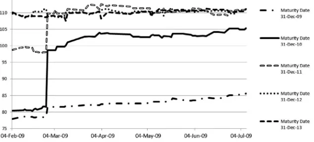
The fair prices of property forwards thus obtained are illustrated in Fig. 3.

A closer examination ofFigs. 2 and 3shows that the jumps in IPD futures and (reversed engineered) forward prices are not contempora-neous, but rather that that futures prices jump up at the end of March, whereas the upward jump in February is visible for the forward prices. While futures prices jump due to the roll-over of the contract at the end of March, forwards–which are reversed engineered based on TRS and UK interest rate data as explained above–jump in February due to jumps in TRS rates, which in turn, should be due to the publication of the new IPD index. This results in the differences between forward and futures, depicted inFig. 4, being higher than usual for almost one month.8

The descriptive statistics of the TRS rates are reported inTable 1. The mean values are mostly negative, signifying that the underlying com-mercial property market will depreciate over the period to the horizon

indicated by the maturity of the contract; the mean for thefirst maturity date is−17.80% and the means are increasing with maturity. The excess kurtosis is negative for allfive futures contracts and thefirst year TRS contract and it is positive for the remaining four series of TRS rates. The skewness values have negative signs, except for the four year fu-tures contract, implying that the distributions of the data are skewed to the left. The descriptive moments of the differences between forward and futures prices on the IPD commercial index are also reported in Table 1. On average, the differences for thefirst three maturities are pos-itive, while for the fourth andfifth maturities they are negative.

It can be seen inTable 1that the futures contract for theﬁfth maturity date appears to have the highest mean. The highest standard deviation is shown in the futures contract for the second maturity date. Similarly to TRS data, futures prices exhibit skewness and fat tail characteristics.

3. Model-free analysis of forward–futures differences

LetS(t) be the spot value of the IPD index at time-t,F(t,Ti), the

asso-ciated time-tforward price with maturityTi,f(t,Ti) the time-tfutures

price with maturityTiandD(t,Ti) the stochastic discount factor at

timetfor maturityTi. ThenB(t,Ti) =EtQ(D(t,Ti)) is the time-t

zero-coupon bond price, with maturityTi, where the expectation is taken

under a risk-neutral measureQ.

There is a model-free relationship between forward and futures prices given by9_:

F tð;TÞ−f tð;TÞ ¼

covQtðS Tð Þ;D tð;TÞÞ EQtðD tð;TÞÞ

ð1Þ

which holds for any maturityTand at any time 0≤t≤T. This funda-mental relationship opens up theﬁrst line of investigation for testing whether the differences between forward and futures prices are statis-tically different from zero.

3.1. Testing methodology

First, the null hypothesis that the difference between the market TRS equivalent forward prices and market futures prices is signiﬁcantly different from zero is tested. If this hypothesis is rejected, then in the second stage a series of models and estimation methods are employed for the terms on the right hand side of the fundamental relationship given by Eq.(1). The aim in the second stage is to decide on the capabil-ity of various models to appropriately capture the dynamics of the index Sand the discount factorD.

Fig. 3.The fair prices of property forwards.Notes: The plotted data is from 4 February to 7 July 2009 for theﬁve maturity datesﬁxed in the market calendar, for the period of study. The fair property forward prices are reversed engineered from the corresponding portfolio of total return swaps.

8

These abnormal forward–futures differences do not drive the signiﬁcance of the re-sults in this paper. The rere-sults remain signiﬁcant even after changing the sample and elim-inating the month of abnormally high forward futures differences. 9

(5)

For theﬁrst stage analysis, the following regression model isﬁtted for each maturity dateTi,i∈{1,2,…,5}:

Fðt;TiÞ ¼α0iþβ0if tð;TiÞ þεti ð2Þ

(withTiﬁxed for each of theﬁve time series regressions) and test

whetherα0i= 0 andβ0i= 1. If the null hypothesis cannot be rejected,

then one can conclude that the difference between forward and futures prices is due to noise. If, however, the null is rejected, we then proceed to the second stage of our analysis. The same econometric analysis de-scribed above from a times series point of view, can also be performed using panel data. Using panel data has a series of advantages.10Firstly, it enables the analysis of a larger spectrum of problems that could not be tackled with cross-sectional or time series information alone. Secondly, it generally results in a greater number of degrees of freedom and a reduction in the collinearity among explanatory variables, thus increasing the efﬁciency of estimation. Furthermore, the larger number of observations can also help alleviate model identiﬁcation or omitted variable problems.

The regression equation in Eq.(2)is rewritten for our panel data as:

F tð;TiÞ ¼α0þβ0f tð;TiÞ þεti ð3Þ

withi∈{1,2,…,5} andt∈{1,2,…,71}.

More variations of a panel regression exist, the simplest one being the pooled regression, described above in Eq.(3), which implies esti-mating the regression equation by simply stacking all the data together, for both the explained and explanatory variables. Furthermore, the

ﬁxed effects model for panel data is given by:

F tð;TiÞ ¼α0þβ0f tð;TiÞ þαiþυit ð4Þ

whereαivaries cross-sectionally (i.e. in our case it is different for each

maturity dateTi), but not over time. Similarly, a time-ﬁxed effects

model can be formulated, in which case one would need to estimate:

F tð;TiÞ ¼α0þβ0f tð;TiÞ þλtþυit ð5Þ

whereλtvaries over time, but not cross-sectionally. Theﬁxed effects

model and the time-fixed effects model, as well as a model withboth fixed effects and the time-fixed effects, will be analyzed. One can test whether thefixed effects are necessary using the redundantfixed effects LR test.

For the panel data random effects model the regression speciﬁcation is given by:

F tð;TiÞ ¼α0þβ0f tð;TiÞ þεiþυit ð6Þ

whereεiis now assumed to be random, with zero mean and constant

varianceσε2, independent ofυitandf(t,Ti). Similarly, a random

time-effects model can be formulated in the context of this paper as:

F tð;TiÞ ¼α0þβ0f tð;TiÞ þεtþυit: ð7Þ

Table 2

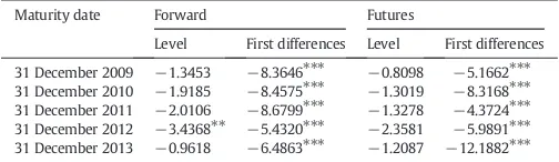
ADF test for the forward and futures prices.

Maturity date Forward Futures

Level First differences Level First differences 31 December 2009 −1.3453 −8.3646⁎⁎⁎ −0.8098 −5.1662⁎⁎⁎ 31 December 2010 −1.9185 −8.4575⁎⁎⁎ −1.3019 −8.3168⁎⁎⁎ 31 December 2011 −2.0106 −8.6799⁎⁎⁎ −1.3278 −4.3724⁎⁎⁎ 31 December 2012 −3.4368⁎⁎ ₋_5.4320⁎⁎⁎ ₋_2.3581 ₋_5.9891⁎⁎⁎ 31 December 2013 −0.9618 −6.4863⁎⁎⁎ ₋_1.2087 ₋_12.1882⁎⁎⁎ Notes: Augmented Dickey–Fuller (ADF) test results for the UK IPD commercial property index forward and futures prices. The test is performed for both the data in levels as well as for thefirst differenced data. The optimum number of lags used in the ADF test equation is based on the Akaike Information Criterion (AIC). The data is from 4 February to 7 July 2009 for thefive maturity dates given in thefirst column.

⁎ _{Denotes signi}_ﬁ_{cance at the 10% level.} ⁎⁎_{Denotes signi}_ﬁ_{cance at the 5% level.}

⁎⁎⁎ _{Denotes signi}_ﬁ_{cance at the 1% level.} 10

See alsoBaltagi (1995),Hsiao (2003).

Fig. 4.The difference between forward and futures prices.Notes: The plotted data is from 4 February to 7 July 2009 for theﬁve maturity datesﬁxed in the market calendar, for the period of study. The fair property forward prices are reversed engineered from the corresponding portfolio of total return swaps.

Table 1

Descriptive statistics for total return swap rates, Eurex futures prices and the forward– futures differences.

Maturity dates

31-Dec-09 31-Dec-10 31-Dec-11 31-Dec-12 31-Dec-13 Total return swaps

Mean −0.178 −0.0971 −0.0389 −0.0056 0.0138 Standard deviation 0.0217 0.0548 0.0521 0.0401 0.0336 Skewness −0.6925 −1.3581 −1.4446 −1.4177 −1.3889 Excess kurtosis −0.5131 0.1383 0.2633 0.2135 0.1585 Futures prices

Mean 81.1982 94.275 106.1732 111.7035 113.5915 Standard deviation 2.6558 10.6358 5.1369 1.2792 3.7762 Skewness −0.0992 −0.4889 −0.5411 0.164 −0.2771 Excess kurtosis −1.5313 −1.7844 −1.6426 −0.6302 −1.6544 Forward–futures differences

(6)

Again, random effects and random time-effects models, as well as a two-way model which allows for both random effects and random time-effects, can be estimated. Furthermore, it is important to test whether the assumption that the random effects are uncorrelated with the regressors is satisﬁed.

For the second stage analysis several models are employed for the dynamics of the IPD indexS. If the analysis is conditioned on knowing the bond prices, the RHS of identity(1)can be expressed as:

covQtðS Tð Þ;D tð;TÞÞ EQtðD tð;TÞÞ

¼ S tð Þ

B tð;TÞ

−EQtðS Tð ÞÞ: ð8Þ

Based on Eqs.(1) and (8), it is evident that for testing purposes the following regression is useful:

F tð;TÞ−f tð;TÞ ¼αþβ S tð Þ

B tð;TÞ

−EQt;mðS Tð ÞÞ

|fflfflfflfflfflfflffl{zfflfflfflfflfflfflffl}

fmðt;TÞ

2

6 4

3

7

5þut;m ð9Þ

and test whetherα= 0 andβ= 1, for each modelm. For each modelm, failing to reject the null hypothesis implies that this particular model is suitable for describing the dynamics of the underlying IPD index. Upon estimation of all the parameters of each modelm,11the regression given in Eq.(9)isfitted. The competing models and methods of estimation are compared with respect to whetherβis significant and also considering the R2measure of goodness-of-fit.

3.2. Model-free analysis

Having both series of forward and futures prices available allows direct testing of whether the forward–futures difference time series diverges signiﬁcantly away from zero. Before running the regressions in Eqs.(2)–(7), the forward and futures price series are tested for stationary using the Augmented Dickey–Fuller (ADF) test. The results are reported inTable 2.

As it can be seen inTable 2, most of the ADF results show that the forward series for thefirst, second, third, andfifth maturity dates are non-stationary while the forward series for the fourth maturity date is stationary at the 5% significance level. In addition, the ADF test indicates that the futures series for all maturity dates are non-stationary. Further-more, the stationarity of thefirst differenced data is also investigated. According toTable 2, the forward and futures series for all maturity dates are stationary in thefirst differences.

Since most of the data is found to be non-stationary in levels and sta-tionary in theﬁrst differences, the remaining analysis is performed on theﬁrst differenced data. The null hypothesis H0:α0i= 0 andβ0i= 1

vs. H1:α0i≠0 orβ0i≠1 is tested using anF-test and the results can

be found inTable 3.

TheF-test results presented inTable 3show that the null hypothesis for all maturity dates could be rejected at the 1% significance level. This implies that the difference between forward and futures is not just noise.12_{The same conclusion is reached if we analyze the values of the} t-statistics for the forward–futures differences reported inTable 4. The results inTable 4show that the significance of the forward–futures difference is not driven by the month of abnormally high differences: in-deed, the difference is still significant when a shorter sample period–2 April to 7 July 2009–is considered, which now eliminates the abnormal sub-period from end February to end March.

As a robustness check of our time-series results, particularly impor-tant given the relatively limited sample available for the time-series analysis (i.e. 71 observations), we also test whether the differences between forward and futures prices are signiﬁcant using a panel regres-sion. To choose an appropriate speciﬁcation for the panel regression, we

ﬁrst test whether theﬁxed effects are necessary using the redundant

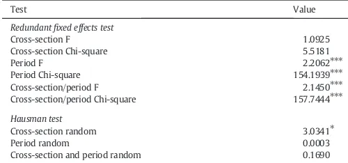
ﬁxed effects LR test. The results of this test are reported inTable 5. From the test results reported inTable 5, it appears that a model with

ﬁxed time effects only is most supported by the data in this research. Furthermore, a random effects model may be appropriate and this is tested using the Hausman test; the results of this test are also reported

11

The speciﬁc stochastic models and parameter estimation methods employed in this paper are described inSection 4below.

Table 3

F-test for time series data.

F-test t-test t-Test

Maturity date α0i= 0 andβ0i= 1 α0i= 0 β0i= 1 Durbin–Watson statistic

31/12/2009 83.5072⁎⁎⁎ 2.2788⁎⁎ −12.9217⁎⁎⁎ 1.9905

31/12/2010 49.4309⁎⁎⁎ 1.3366 −9.9426⁎⁎⁎ 2.0595

31/12/2011 23.8320⁎⁎⁎ 1.1492 −6.9033⁎⁎⁎ 2.0613

31/12/2012 31.1717⁎⁎⁎ _0.1737 ₋_7.8919⁎⁎⁎ _2.2589

31/12/2013 158.2534⁎⁎⁎ _0.2345 ₋_17.7483⁎⁎⁎ _2.7247

Notes:F-Test t-test and Durbin–Watson statistic results for the regression in the Eq.(2)for the property forward and futures data from 4 February until 7 July 2009 for theﬁve maturity dates given in theﬁrst column. For theF-test, the null hypothesis is that the difference between the forward and futures prices is just noise (i.e.α0i= 0 andβ0i= 1).

⁎ _{Denotes signi}_fi_{cance at the 10% level.} ⁎⁎ _{Denotes signi}_fi_{cance at the 5% level.} ⁎⁎⁎ _{Denotes signi}_fi_{cance at the 1% level.}

12

In addition, the diagnostic statistics for these regressions are investigated and the Durbin–Watson test statistic results are reported inTable 3. For all but thefifth maturity date there is no autocorrelation in the regression errors. Furthermore, the individual t-tests for the individual hypothesesα0i= 0 (vs.α0i≠0) andβ0i= 1 (vs.β0i≠1) are also reported. Wefind thatβis always different from 1 and thatαis generally not different from zero (with the exception of thefirst maturity).

Table 4

t-Statistics for the differences between forward and futures prices.

t-Statistic Maturity dates

31-Dec-09 31-Dec-10 31-Dec-11 31-Dec-12 31-Dec-13

4 Feb–7 Jul 2009 6.7060⁎⁎⁎ _4.9265⁎⁎⁎ _4.6852⁎⁎⁎ ₋_12.741⁎⁎⁎ _10.1291⁎⁎⁎

2 Apr–7 Jul 2009 6.695⁎⁎⁎ 6.826⁎⁎⁎ 4.612⁎⁎⁎ −20.003⁎⁎⁎ −20.261⁎⁎⁎

Notes: The values of thet-test are computed for the differences between forward and futures prices on the UK IPD commercial property index, using data from 4 February to 7 July 2009 and from 2 April to 7 July, respectively, for theﬁve maturity dates given in the second row.

(7)

inTable 5. Based on these results, the random effect model is to be preferred in this case.

Next, theF-test statistic for multiple coefﬁcient hypotheses is com-puted using the panel regression random effect speciﬁcation; the results are reported inTable 6.

According toTable 6, theF-values are signiﬁcant at the 1% level. The null hypothesis (H0:α0= 0 andβ0= 1) can be strongly rejected and

therefore the differences between forward and futures are not just noise in the panel data.13

4. Analysis with parametric models

Having shown in the previous section that IPD forward–futures price differences are statistically signiﬁcant, one-factor and two-factor mean-reverting models that seem suitable for this asset class are studied in this section. The models are subsequently coupled with two different methods of parameter estimation–maximum likelihood (ML) as well Markov Chain Monte Carlo (MCMC) for which various quantiles from the distribution of parameters are esti-mated–the model parameters are calibrated to IPD index data, the modelfutures and forward prices are thus calculated andﬁnally, a number of statistical tests are implemented in order to see which model and estimation method best captures the empirical evolution of the IPD forwards and futures.

4.1. Mean-reverting models

Here a slight variation of the trending (mean-reverting) OU process presented inLo and Wang (1995)is considered as follows: letp(t) = ln(S(t));p(t) =q(t) + (μ0+μt),14where the dynamics

ofq(t) under the physical measurePare described by the equa-tion:

for any 0≤t≤T, where the model parameters will be estimated (using both maximum likelihood and MCMC) using the IPD index data, as detailed below. The model-implied (theoretical) futures price can be now be derived in closed-form as outlined inAppendix A:

funivð0;TÞ ¼

whereηis the market price of risk, which shall be calibrated following standard practice, by minimizing the squared difference between the market and model (theoretical) futures prices.

As remarked inLo and Wang (1995), although this speciﬁcation is a valid modeling starting point, it has an important disadvantage in that the autocorrelation coefﬁcients of continuously compoundedτ-period returns can only take negative values.15_{A more}

ﬂexible approach, also proposed inLo and Wang (1995), is the bivariate trending OU process, a natural extension of the univariate version above.

We propose the following version of their bivariate model, to suit the application in this paper:

dq tð Þ ¼½−γq tð Þ þλr tð ÞdtþσdWSð Þt ð13Þ

dr tð Þ ¼δ μð r−r tð ÞÞdtþσrdWrð Þt ð14Þ

wheredWS(t)dWr(t) =ρdtand the second stochastic factor on which

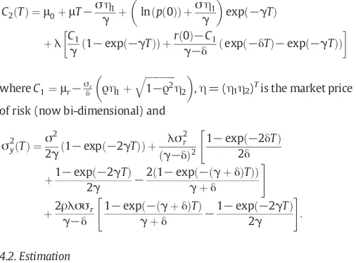
the log-price of the underlying depends is the short interest rater(t).16 Following the derivations and risk neutralization performed in Appendix B, the futures price is obtained in closed form:

fbivarð0;TÞ ¼ exp C2ð Þ þT

TheF-test for panel data.

Test statistic Value

F-statistic 237.3960⁎⁎⁎

Durbin–Watson statistic 2.1419

Notes:F-test and Durbin–Watson statistic results for the regression in Eq.(6)for the prop-erty forward and futures panel data from 4 February to 7 July 2009, using the cross-section random effects speciﬁcation. For theF-test, the null hypothesis is that the difference between the forward and futures prices is just noise (i.e.α0= 0 andβ0= 1).

⁎ _{Denotes signi}_fi_{cance at the 10% level.} ⁎⁎_{Denotes signi}_fi_{cance at the 5% level.} ⁎⁎⁎ _{Denotes signi}_fi_{cance at the 1% level.}

13_{In addition, the values of the Durbin}_–_{Watson test show that there is no}

autocorrela-tion in the panel regression errors.

14

To simplify notation, we suppress model subscripts,univandbivarfor the univariate and bivariate models, respectively, unless where absolutely necessary.

15

The continuously compoundedτ-period returns, computed at timet, are deﬁned as rτ(t) =p(t)−p(t−τ). The autocorrelation function of the returns process employed here is the same as inLo and Wang (1995)–see their expression (A3)–namely:

corrunivðrτð Þ;t1 rτð Þt2Þ ¼−

1

2exp½−γðt2−t1−τÞ½1−expð−γτÞ2≤0;

for anyt1,t2, andτsuch thatt1≤t2−τ, to ensure that returns are non-overlapping. 16_{The expression for the correlation of}_τ_{-period returns}_corr

bivar(rτ(t1),rτ(t2)) for anyt1,

t2, andτsuch thatt1≤t2−τ, is mathematically more complex and thus excluded here.

However, it can be shown that for certain values of the model parameters, the bivariate model, unlike the univariate model outlined above, is moreﬂexible and can allow for both positive and negative autocorrelations.

Table 5

Tests for determining the most suitable panel regression model.

Test Value

Cross-section and period random 0.1690

Notes: The redundantfixed cross-section effects test has a panel regression withfixed time (period) effects only under the null. Both theFand the Chi-square version of the test are reported. The redundantfixed time (period) effects have a panel regression withfixed cross-section effects only under the null. Both theFand the Chi-square version of the test are reported. For the random effects test (i.e. Hausman test) the null hypothesis in this case is that the random effect is uncorrelated with the explanatory variables. The panel data is from 4 February to 7 July 2009 forfive maturities, namely December 2009, December 2010, December 2011, December 2012 and December 2013.

(8)

with

of risk (now bi-dimensional) and

σ2yð Þ ¼T

In order to be able to use the models enumerated above their param-eters should be calibratedﬁrst. The parameters of the continuous time models speciﬁed in Eq. (10) and Eqs.(13)–(14)can be estimated from the monthly log prices on the IPD index, observed over the period be-tween December 1986 and January 2009, and totalling 266 historical observations. The estimates then will be carried forward for analyzing the differences between the forward and futures on IPD starting from February 2009.

4.2.1. Maximum likelihood

When feasible, parametric inference for diffusion processes from discrete-time observations should employ the likelihood function, given its generality and desirable asymptotic properties of consistency and efﬁciency (Phillips & Yu, 2009). The continuous time likelihood function can be approximated with a function derived from discrete-time observations, obtained by replacing the Lebesgue and Ito integrals with the Riemann–Ito sums. Remark that this approach gives reliable

results only when the observations are spaced at small time intervals. When the time between observations is not small the maximum likeli-hood estimator can be strongly biased inﬁnite samples.17

First de-trend the log price data by estimating the regression:

ptk¼μ0þμtkþutk ð16Þ

and subsequently work with the residuals from this equation, where k= 1, 2,…, 266 andtk=kτ, withτ¼121 for monthly returns. The

(exact) discretization of Eq.(11)leads to:

utk¼cutk−1þεtk ð17Þ

Maximum likelihood estimation of the discrete-time model in Eq.(17)gives18_c_{= 0.995086 and the standard deviation of}

εtkas 0.011. The exact discretization of the two-factor model given by Eqs.(B.7)–(B.8)(given inAppendix Bfor lack of space) is:

qtk¼αqþβqqtk−1þφrtk−1þεq;tk rtk¼αrþβrrtk−1þεr;tk

ð18Þ

where, for reasons of space, the expressions for the parameters as well as the distribution of the error terms in Eq.(18)are only given in Appendix C.

4.2.2. Markov Chain Monte Carlo (MCMC)

Despite its desirable asymptotic properties, ML estimates of the pa-rameters of a continuous-time model based on discrete-sampled data

17 _{Further discussion is given in}_{Dacunha-Castelle and Florens-Zmirou (1986)}_,_Lo (1988),Florens-Zmirou (1989),Yoshida (1990)andPhillips and Yu (2009).

18

To check the stability of the parameter estimates, the estimation above is repeated using a larger sample, namely Dec 1986 to Oct 2010, with an increased sample size of 287 monthly observations. The parameter estimates do not change much.

Table 7

Models and estimation methods.

Name Model Estimation method

univ_ML Univariate time-trending OU:dq(t) =−γq(t)dt+σdW(t) Exact maximum likelihood

univ_MCMC_mean Markov Chain Monte Carlo (MCMC), mean parameter estimates

univ_MCMC_2.5q MCMC, using the 2.5th quantile of the distribution of estimates

univ_MCMC_97.5q MCMC, using the 97.5th quantile of the distribution of estimates

bivar_ML Bivariate time-trending OU:

dq tð Þ ¼½−γq tð Þ þλr tð ÞdtþσdWSð Þt dr tð Þ ¼δ μð r−r tð ÞÞdtþσrdWrð Þt dWSð ÞtdWrð Þ ¼t ρdt

Exact maximum likelihood

biv_MCMC_mean MCMC, mean parameter estimates

biv_MCMC_2.5q MCMC, using the 2.5th quantile of the distribution of estimates

biv_MCMC_97.5q MCMC, using the 97.5th quantile of the distribution of estimates

Notes:q(t) is the de-trended log price process for the underlyingS(t), the IPD UK commercial property price index:p(t) = ln(S(t));p(t) =q(t) + (μ0+μt).r(t) denotes the short

in-terest rate. For both models, the futures price is obtained as:fm(0,T) =E0,Qm(S(T)) wherem=univorbivar, for the two models, respectively,Qis the martingale pricing measure, and Tis the futures maturity time.

Table 8

Parameter estimates.

Parameter/model univ_ML univ_MCMC_mean univ_MCMC_2.5q univ_MCMC_97.5q

μ0 – 4.221 1.35 4.463

μ 0.4117 0.3121 0.2657 0.7051

γ 0.0591 1.559 0.1892 1.979

σ 0.0384 0.0178 0.0131 0.0238

η(average) −37.2076 −962.8572 −259.2317 −944.3792

(9)

are biased inﬁnite samples. An alternative estimation technique that is applied here in order to circumvent this problem is the Markov Chain Monte Carlo (MCMC) methodology (seeTsay, 2010).

MCMC techniques19are based on a Bayesian inference theoretical support and offer an elegant solution to many problems encountered with other estimation methods, at the cost of computational effort. The main advantage of employing this type of inferential mechanism is the capability to produce not only a point estimate but an entire pos-terior distribution for parameters of interest. Selecting various statistics from this distribution provides a more informed view on the plausible values of the parameters. Hence, for estimation purposes the mean, the 2.5% quantile and the 97.5% quantile of the posterior distribution of the mean reversion parameter are going to be used. The estimates for the discretized version of the mean-reverting model given in Eq.(10)are reported inTable 8. One great advantage of the MCMC

approach is that all parameters are estimated easily from the same output without additional computational effort.

4.3. The calibration of the market price of risk

To calibrate the market price of riskη, we compute the differences (i.e. pricing errors) between observed and model futures prices. Subse-quently, standard practice is followed and the value ofηis chosen such that it minimizes the mean squared error function. This optimization exercise is performed for each day in our sample and for each of the estimation methodologies described above. All parameter estimates can be determined now and then the theoretical model can be used for producing property futures prices.Table 7gives a list of the models investigated in this paper with various methods of estimation. In Table 8we report the parameter estimation results forﬁrst half of these models based on our data.20

19

For an excellent introduction seeTsay (2010). All MCMC inference in this paper has been produced with WinBUGS 1.4, from a sample of 100,000 iterations after a burn-in pe-riod of 500,000 iterations.

20

Due to lack of space, the empirical implementation of the bivariate models is left for future research.

Table 9

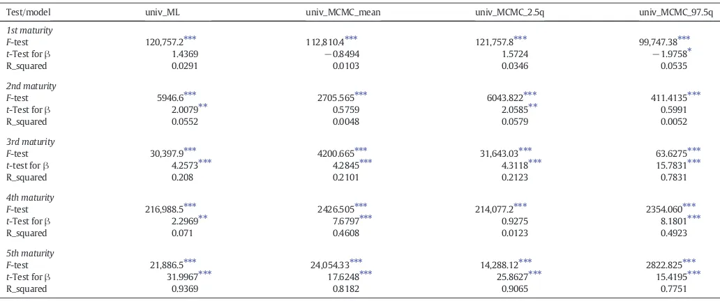
Model comparison—time series data.

Test/model univ_ML univ_MCMC_mean univ_MCMC_2.5q univ_MCMC_97.5q

1st maturity

F-test 120,757.2⁎⁎⁎ 112,810.4⁎⁎⁎ 121,757.8⁎⁎⁎ 99,747.38⁎⁎⁎

t-Test forβ 1.4369 −0.8494 1.5724 −1.9758⁎

R_squared 0.0291 0.0103 0.0346 0.0535

2nd maturity

F-test 5946.6⁎⁎⁎ 2705.565⁎⁎⁎ 6043.822⁎⁎⁎ 411.4135⁎⁎⁎

t-Test forβ 2.0079⁎⁎ 0.5759 2.0585⁎⁎ 0.5991

R_squared 0.0552 0.0048 0.0579 0.0052

3rd maturity

F-test 30,397.9⁎⁎⁎ 4200.665⁎⁎⁎ 31,643.03⁎⁎⁎ 63.6275⁎⁎⁎

t-test forβ 4.2573⁎⁎⁎ 4.2845⁎⁎⁎ 4.3118⁎⁎⁎ 15.7831⁎⁎⁎

R_squared 0.208 0.2101 0.2123 0.7831

4th maturity

F-test 216,988.5⁎⁎⁎ 2426.505⁎⁎⁎ 214,077.2⁎⁎⁎ 2354.060⁎⁎⁎

t-Test forβ 2.2969⁎⁎ 7.6797⁎⁎⁎ 0.9275 8.1801⁎⁎⁎

R_squared 0.071 0.4608 0.0123 0.4923

5th maturity

F-test 21,886.5⁎⁎⁎ 24,054.33⁎⁎⁎ 14,288.12⁎⁎⁎ 2822.825⁎⁎⁎

t-Test forβ 31.9967⁎⁎⁎ 17.6248⁎⁎⁎ 25.8627⁎⁎⁎ 15.4195⁎⁎⁎

R_squared 0.9369 0.8182 0.9065 0.7751

Notes: For the regression in Eq.(9), we report the value of theF-statistics for the nullα= 0 andβ= 1, the value of thet-statistic for the beta coefficient and the R-squared of the regres-sion, where the RHS, independent variable is based on the univariate OU model with parameters estimated using maximum likelihood (ML) in column 2 and Markov Chain Monte Carlo (MCMC) in columns 3–5, with mean (column 3), 2.5th quantile (column 4) and 97.5th quantile (column 5) parameter estimates. The data used forfitting the model parameters with these alternative estimation methods contains monthly log prices on the IPD index, observed over the period between December 1986 and January 2009, and totalling 266 historical observa-tions. The forwards and futures data used for the testing reported in this table is from 4 February to 7 July 2009 forfive maturities, namely December 2009, December 2010, December 2011, December 2012 and December 2013.

⁎ _{Denotes signi}_fi_{cance at the 10% level.} ⁎⁎ _{Denotes signi}_fi_{cance at the 5% level.} ⁎⁎⁎ _{Denotes signi}_fi_{cance at the 1% level.}

Table 10

Model comparison—panel data.

Test/model univ_ML univ_MCMC_mean univ_MCMC_2.5q univ_MCMC_97.5q

F-test 62,789.3⁎⁎⁎ 26,358.31⁎⁎⁎ 64,035.43⁎⁎⁎ 10,284.18⁎⁎⁎

t-Test forβ 10.7141⁎⁎⁎ 11.3375⁎⁎⁎ 10.6135⁎⁎⁎ 6.8171⁎⁎⁎

R_squared 0.2454 0.2669 0.2419 0.1163

Notes: For the regression in Eq.(9), we report the value of theF-statistics for the nullα= 0 andβ= 1, the value of thet-statistic for the beta coefficient and the R-squared of the regres-sion, where the RHS, independent variable is based on the univariate OU model with parameters estimated using maximum likelihood (ML) in column 2 and Markov Chain Monte Carlo (MCMC) in columns 3–5, with mean (column 3), 2.5th quantile (column 4) and 97.5th quantile (column 5) parameter estimates. The data used forfitting the model parameters with these alternative estimation methods contains monthly log prices on the IPD index, observed over the period between December 1986 and January 2009, and totalling 266 historical observa-tions. The panel forwards and futures data used for the testing reported in this table is from 4 February until 7 July 2009, forfive maturities, namely December 2009, December 2010, De-cember 2011, DeDe-cember 2012 and DeDe-cember 2013.

(10)

4.4. Empirical results

The empirical analysis considers here a more refined investiga-tion looking at several models for the underlying IPD index dynam-ics, coupled with a model for interest rates, but also considering several estimation methods. From afinancial economics point of view, it has been established that even if the interest rates are con-stant then futures prices can differ from the associated forward prices. Assuming that interest rates are stochastic leads directly to the conclusion that the two series will diverge significantly over time. In this part of the paper the research question is “which model and estimation method most likely support the observed mar-ket differences?”Furthermore, an additional level of complexity is generated from employing panel data tests.

Tables 9 and 10summarize the results of our model comparison, for the time series and panel data, respectively. The MCMC methods perform better than the ML method. The R-square seems to increase with maturity overall hinting that stationarity problems may be more acute for near maturities. Please note that since maturities areﬁxed in the calendar by the market, the time to maturity of our series gets progressively smaller, across allﬁve contracts.

The results inTable 10reveal that for panel data analysis all models employed here are well speciﬁed and the betat-test is highly signiﬁcant. All models apart from the MCMC approach for the 97.5th quantile yield similar values for the R-squared, of around 20%.

5. Conclusions

In this paper the differences between forward and futures prices are analyzed on commercial real-estate, using a battery of models, estimation methods and tests. The forward prices have been reversed engineered from total return swap rates using standard market practice. Testing is done not only on individual time series data but also in a panel data framework.

The results obtained in this paper provide evidence of signiﬁcant differences between the implied forward and futures prices for the IPD UK index. One possible explanation could be the period of study, several months during 2009, in the aftermath of the subprime crisis.

Although the overall conclusion is that, for the period 4 February 2009 to 7 July 2009, the forward prices were different from futures prices, there is substantial variation in the strength of these results across contract maturities, methods of estimation and testing frame-works. Given the significance of these results on a model-free basis ini-tially, a model race that best explains the relationship between synthetic forward prices derived from daily total return swap rates and the daily futures prices was performed. The models were generated by using various methods of estimation for the mean-reverting OU continuous time process assumed for the underlying IPD index. The models employed in the paper provided significant explanatory power for the relationship between forward and futures prices on commercial real-estate index in the UK but the analysis of the error terms shows that there is more that can be explained. From a theoretical point of view our study can be expanded to more advanced two-factor models as detailed in the paper. The difficult question to answer then is what constitutes the second factor for commercial-real estate. This would be the subject of a future research.

Acknowledgement

We are very grateful to Eurex for supporting our research and providing us with the data on IPD UK futures. We would also like to thank an anonymous referee for very helpful suggestions which helped improve the paper. All mistakes are obviously ours.

Appendix A. The derivation of the futures price for the univariate process

Using Eq. (10), the corresponding equation forp(t) under the real-measurePis:

dp tð Þ ¼½μ−γðp tð Þ−ðμ0þμtÞÞdtþσdW tð Þ;

and upon risk neutralization it becomes:

dp tð Þ ¼½μ−γðp tð Þ−ðμ0þμtÞÞ−ησdtþσdW

Q t

ð Þ

whereηis the market price of risk andWQ(t) is a Q-Brownian motion. The solution to this modiﬁed equation is similar to Eq.(11):

p tð Þ ¼μ0þμt−μ0expð−γtÞ− theoretical futures prices can be obtained in closed-form, as given in Eq.(12):

Appendix B. The derivation of the futures price for the bivariate process

The solution to Eq.(14)is:

r tð Þ ¼μrþexpð−δtÞðrð Þ0−μrÞ þσr

Zt

v¼0

expð−δðt−vÞÞdWrð Þv ðB:1Þ

for any 0≤t≤T. Combining Eqs.(B.1)and (13) gives the analytical solution for the log of the underlying index value:

p tð Þ ¼μ0þμtþexpð−γtÞðpð Þ0−μ0Þ þ

Next, in order to obtain the risk neutralQ-dynamics of the system in Eqs.(13) and (14)wheredWS(t)dWr(t) =ρdtﬁrst the system is

rewrit-ten under the physical measureP, but depending solely on the non-correlated Brownians21W1andW2, where, for anyt

W1ð Þ ¼t WSð Þt

(11)

Wrð Þ ¼t ϱW1ð Þ þt ffiffiffiffiffiffiffiffiffiffiffiffiffi

1−ϱ2 q

W2ð Þt : ðB:4Þ

Thus, the system in Eqs.(13)–(14)can be re-written as follows:

dp tð Þ

The risk neutralQ-dynamics of this system is given by:

dp tð Þ

The above system can be solved leading to the solution:

r tð Þ ¼C1þ½r sð Þ−C1expð−δðt−sÞÞ þσr

Zt

v¼s

expð−δðt−vÞÞdWQrð Þv:

ðB:7Þ

Or, slightly simpliﬁed,

r tð Þ ¼C1þ½rð Þ0−C1expð−δtÞ þσr

The futures price for maturityTcan be easily derived now as:fbivar(0,T) =

E0,Qbivar(S(T)) and calculations of this expectation yield the expression in

Eq.(15).

Appendix C. The discretization of the bivariate model

The complete speciﬁcation of the discretization for the two-factor model used in the paper is given as

qtk¼αqþβqqtk−1þφrtk−1þεq;tk

The error vector is bivariate normal, with covariance matrix22_:

var εq;tk

Eqs. (C3) and (C5) represent a system of two equations in two unknowns,σandρ.

Appendix D. Maximum likelihood estimation—continuous time models parameters in terms of the discrete time models parameters

Univariate model

(12)

References

Alles, L. A., & Peace, P. P. K. (2001).Futures and forward price differential and the effect of marking-to-market: Australian evidence.Accounting and Finance,41, 1–24. Baltagi, B. H. (1995).Econometric analysis of panel data.Chichester: Wiley.

Bjork, T. (2009).Arbitrage theory in continuous time (3rd ed.). Oxford: Oxford University Press.

Case, K. E., & Shiller, R. J. (1989).The efﬁciency of the market for single family homes.

American Economic Review,79, 125–137.

Case, K. E., & Shiller, R. J. (1990).Forecasting prices and excess returns in the housing market.AREUEA Journal,18, 253–273.

Case, K. E., & Shiller, R. J. (1996).Mortgage default risk and real estate prices: The use of index based futures and options in real estate.Journal of Housing Research,7, 243–258.

Case, K. E., Shiller, R. J., & Weiss, A. N. (1993).Index-based futures and options trading in real estate.Journal of Portfolio Management,19, 83–92.

Cornell, B., & Reinganum, M. R. (1981).Forward and futures prices: Evidence from the foreign exchange markets.Journal of Finance,36, 1035–1045.

Cox, J. C., Ingersoll, J. E., & Ross, S. A. (1981).The relation between forward prices and futures prices.Journal of Financial Economics,9, 321–346.

Dacunha-Castelle, D., & Florens-Zmirou, D. (1986).Estimation of the coefﬁcients of a diffusion from discrete observations.Stochastics,19, 263–284.

Fabozzi, F. J., Shiller, R., & Tunaru, R. S. (2012).A pricing framework for real-estate derivatives.European Financial Management,18, 762–789.

Fisher, J.D. (2005).New strategies for commercial real estate investment and risk management.Journal of Portfolio Management,32, 154–161.

Florens-Zmirou, D. (1989).Approximate discrete-time schemes for statistics of diffusion processes.Statistics,20, 547–557.

French, K. R. (1983).A comparison of futures and forward prices.Journal of Financial

Economics,12, 311–342.

Grinblatt, M., & Jegadeesh, N. (1996).Relative pricing of Eurodollar futures and forward contracts.Journal of Finance,51, 1499–1522.

Hsiao, C. (2003).Analysis of panel data(2nd ed.). Cambridge: Cambridge University Press. Jarrow, R. A., & Oldﬁeld, G. S. (1981).Forward and futures contracts.Journal of Financial

Economics,9, 373–382.

Kane, E. J. (1980).Market incompleteness and divergences between forward and futures interest rates.Journal of Finance,35, 221–234.

Levy, A. (1989).A note on the relationship between forward and futures contracts.Journal

of Futures Markets,9, 171–173.

Lo, A. W. (1988).Maximum likelihood estimation of generalized Ito processes with discretely sampled data.Econometric Theory,4, 231–247.

Lo, A. W., & Wang, J. (1995).Implementing option pricing models when asset returns are predictable.Journal of Finance,50, 87–129.

Margrabe, W. (1978).A theory of forward and futures prices.Working paper. Philadelphia: The Wharton School, University of Pennsylvania.

Meulbroek, L. (1992).A comparison of forward and futures prices of an interest rate-sensitiveﬁnancial asset.Journal of Finance,47, 381–396.

Morgan, G. (1981).Forward and futures pricing of treasury bills.Journal of Banking and

Finance,5, 483–496.

Park, H. Y., & Chen, A. H. (1985).Differences between futures and forward prices: A further investigation of the marking-to-market effects.Journal of Futures Markets,5, 77–88.

Phillips, P. C. B., & Yu, J. (2009).Maximum likelihood and Gaussian estimation of contin-uous time models inﬁnance. In T. G. Andersen, R. A. Davis, J. Kreiβ, & T. Mikosch (Eds.),Handbook ofﬁnancial time series. New York: Springer.

Polakoff, M. (1991).A note on the role of futures indivisibility: Reconciling the theoretical literature.Journal of Futures Markets,11, 117–120.

Polakoff, M., & Diz, F. (1992).The theoretical source of autocorrelation in forward and futures price relationships.Journal of Futures Markets,12, 459–473.

Richard, S., & Sundaresan, M. (1981).A continuous time equilibrium model of forward prices and futures prices in multigood economy.Journal of Financial Economics,9, 347–392.

Shiller, R. J. (2008).Derivatives markets for home prices.Cambridge Massachusetts: Nation-al Bureau of Economic Research.

Shiller, R. J., & Weiss, A. N. (1999).Home equity insurance.Journal of Real Estate Finance

and Economics,19, 21–47.

Shreve, S. E. (2004).Stochastic calculus forﬁnance II: Continuous-time models.NewYork: Springer.

Tsay, R. (2010).Analysis ofﬁnancial time series (3rd ed.). New York: Wiley.

Wimschulte, J. (2010).The futures and forward price differential in the Nordic electricity market.Energy Policy,38, 4731–4733.

Yoshida, N. (1990).Estimation for diffusion processes from discrete observations.Journal