The Transform between Geographic Coordinates and Location Codes of Aperture 4
Hexagonal Grid System
Wang Ruia,*, Ben Jina,b, Li Yalua, Du Lingyua
a Institute of Surveying and Mapping, Information Engineering University, Zhengzhou 450052, China- [email protected], [email protected], [email protected], [email protected]
b State Key Laboratory of Resource and Environmental Information System, Chinese Academy of Science, Beijing 100101, China,
KEY WORDS: Discrete Global Grid System, Location Code, Geographic Coordinate, Conversion, Code Operation
ABSTRACT:
Discrete global grid system is a new data model which supports the fusion processing of multi-source geospatial data. In discrete global grid systems, all cell operations can be completed by codes theoretically, but most of current spatial data are in the forms of geographic coordinates and projected coordinates. It is necessary to study the transform between geographic coordinates and grid codes, which will support data entering and getting out of the systems. This paper chooses the icosahedral hexagonal discrete global system as a base, and builds the mapping relationships between the sphere and the icosahedron. Then an encoding scheme of planar aperture 4 hexagonal grid system is designed and applied to the icosahedron. Basing on this, a new algorithm of transforms between geographic coordinates and grid codes is designed. Finally, experiments test the accuracy and efficiency of this algorithm. The efficiency of code addition of HLQT is about 5 times the efficiency of code addition of HQBS.
1. INTRODUCTION
Discrete Global Grid Systems (DGGS) is a new global-oriented data model, of which the main characteristic is the digital representation of geospatial location. DGGS partition the globe into uniform grid cells in hierarchical structure and address every cell using location code to substitute for traditional geographic coordinates in operation. Compared with the traditional spatial data models, DGGS take the globe as the research object and provide worldwide uniform space datum. Each grid cell is correspond to one geographical location and cell size will change in terms of the level of grid, which help process of multi-resource, isomerous and multi-resolution geospatial data. Moreover, in DGGS, geometrical operation of grid cells can be achieved completely by location codes which improve efficiency of data computation and process.1
Common cell shapes used by DGGS are triangles, quadrangles and hexagons. Compared with other two shapes, the topological relationship of hexagonal grids is consistent, which is beneficial
*Corresponding author at: Information Engineering University, Zhengzhou 450052, China
E-mail address: [email protected]
for spatial analysis like adjacency and connection (Sahr et al., 2003; Ben et al., 2015a). Spatial sampling efficiency of hexagonal grids is highest and helps data visualization (Sahr, 2011). The processing efficiency of sampling values is about 20 percent to 50 percent higher than quadrangles (Sahr, 2011).
Corporation in Canada developed the spatial data integration software based on the ISEA3H grid system and its core technology is PYXIS grid indexing patent (Peterson, 2006).
Although current research has made considerable progress, some deficiency exists. In the PYXIS scheme, the direction of grid cells will change with levels of resolution, which is not beneficial to spatial analysis like adjacency. The concept model of HQBS is so complicated that there are frequent failure in code regularization and operaions will rollback, which seriously affects computational efficiency. The operations of cells can be completely realized by location code in grid systems, but at present most spatial data are still represented and stored in the form of traditional geographic coordinates or projection coordinates. To ensure that spatial data can transform between the traditional data organization framework and grid systems at a high speed, it is necessary to make research on conversion between geographic coordinates and location codes.
Above all, this paper chooses the icosahedral DGGS and firstly establishes the mapping relationship between the regular icosahedron and the sphere. Then, an encoding scheme of the planar aperture 4 hexagonal grid system is designed and applied into the icosahedron skillfully. Based on this, we desinged a new algorithm of conversion between geographic coordinates and location codes of grids and compares with the scheme HQBS to verify validity and high efficicency of the algorithm.
2. LOCATION OF THE REGULAR ICOSAHEDRON
AND MAPPING RELAITON WITH THE SPHERE
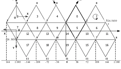
In order to establish the mapping relation between the surface of a regular icosahedron and the sphere, firstly we should determine the location relationship between the regular icosahedron and the earth spheriod. Locate two vertices of the regular icosahedron at the north and south poles respectively and locate another one vertex at (0±;25:56505±N ). Then
flatten the regular icosahedron and number each vertex or assign every vertxe an index as illustrated in Figure 1. The rule is as the following: Vertex located at the North pole and South pole are indexed as 0 and 11 respectively. The number 1 vertex is at the baisi meridian and the restcan be done in the same manner. Apart from vertices, faces are needed to be indexed as well: faces north of
25:56505
±N
are assigned 0-4 and facesfaces south of
25:56505
±S
assigned 15-19 and faces sharingcommon edges with them are assinged 10-14. According to the above relations, given a point P (B ;L ) whose geograohic coordinates, that is longitute and latitude, is known, the index
T
P of the triangular face P (B ;L ) belongs to can be obtained.For the projection between the regular icosahedron and the sphere, this paper adopts Snyder Equal-area Map Projection for polyhedral globes to establish the mapping relations of single face of the icosahedron and the sphere. The Snyder projection ensures the continuity of network of longitude and latitude and decrease the distortion at the same time. The forward and inverse solution, detailed procedure and algorithms of Snyder Equal-area Map Projection can be referenced in Snyder (1992) and Ben et al. (2006) but not discussed in this paper.
In terms of the above location and projection, given a point
P (B ;L ), compute the triangular face number
T
P it locates at,then via Snyder projection, the 2D Cartesian coordinate
p(xp;yp) of
P
in the triangular face can be obtained. Herein introduce the coordinate systemO
X Y
in triangular face as shown in Figure 1. The originO
is at the centroid of the regular face. Face indexed as 0-4 and 0-14 are called ‘ Up Triangular Face’ whose directions of axis are the same as Face 2. Similarly, Face 5-9 and Face 15-19 are called ‘ Down Triangular Face’, whose directions of axis are the same as Face 7. Hence, conversion between geographic coordinates and locaiton codes are simplified into a single triangular face.N
0 0 0 0
11 11
144 ± 180 - 144 - 108 - 72 - 36 0 36 72 108 144 ± 180
11 11 11
0
4 5 1 2 3
8 9 10 6 7 8
3 4 0 1
6 10 5 14 9 13 8 12 7
17 18 19 15 16
3
N
26. 5650 5
- 26. 56505
2
11
Y
X
X
Y O
O
Figure 1. Indexes of vertices and faces in the icosahedron and the coordinate system in triangular face
3. ENCODING OF THE A4H
Above analysis, in order to complete the conversion, we need to research relationship between locaiton codes on the triangular faces and the correspongding 2D Cartesian coordinates. Centers of grid cells are called lattice, which are identified with grid cells in our research. For convnence of code substitution, this paper adopts complex numbers to represent lattice locations (Vince, 2006a, 2006b). Thereinaftet, let
n
denote the partition level of grids, and the higher the level, the finer the resolution or the size of grid cell. According to geometry of the aperture 4 hexagongal grid system (A4H), lattice at leveln
, n > 1, comprises lattice and midpoints of each cell edges at leveln
1
.where ‘
P
’ and ‘+’ mean accumulation among sets.In equation (1), representation of each lattice is unique, which satifies the requirement of the location code for uniqueness. Let
x = :d1d2 dn(d1 2 D0;d2; ;dn 2 D ) denote
x 2 L
n;n > 1
,d
1,d
2,…dn
are all complex numbers so it is not convenient for expression and computation. Now, replaced
i, 1 6 i 6 n, with location codes. Omit the base of powerexponents in equation (1) and make replacement as below
d1 = !0e! e(1 6 e 6 6);di= !e! e(1 6 e 6 3; convenience of representation, thereinafter name the hierarchical structure of lattice of A4H Hexagonal Lattice Quad Tree (HLQT).
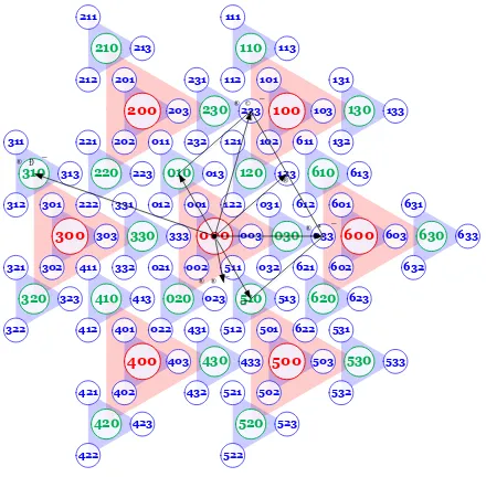
Figure 2. Representation of codes in the 3rd level and examples of code operation
233
000 = 233
. For the inverse element, 010510 = 0;
510 = 010
. For the property (5), 010 123 =.123 010 = 233. And these properties make G fHn; g the Abelian group.The operation rule of code addtion is similar to the decimal addition essentailly. In operation , we reference the addition table as Table 1.
Table 1. Addition table of seven code cells
0 1 2 3 4 5 6
0 0 1 2 3 4 5 6
1 1 100 20 2 0 6 10
2 2 20 200 30 3 0 1
3 3 2 30 300 40 4 0
4 4 0 3 40 400 50 5
5 5 6 0 4 50 500 60
6 6 10 1 0 5 60 600
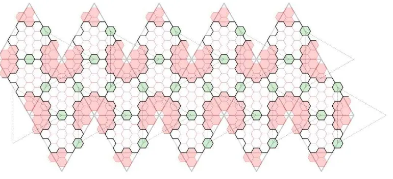
3.2 Extend of the encoding scheme onto the icosahedron
Hereinbefore, we discussed the encoding scheme on the infinite 2D plane, but the surface of the regular icosahedron is closed. In order to extend the encoding scheme to the regular icosahedron, ‘face tile’ and ‘vertex tile’ are used to depict its structure. The flattened icosahedron is shown in Figure 3. The face tiles are centered at the center of each triangle of the icosahedron and the cells of them are filled in white. The vertex tiles are centered at the center of each vertex of the icosahedron and the cells of them are filled in red and green.
Denote the set of lattice of the icosahedral A4H at level n
Gn(n > 1).
G
n comprises two parts. One part is 20 facetiles Ai
n;i = 0;1; ;19 and i is the index of the triangular faces the face tile is centered at. Another part is 12 vertxe tiles Vj
n;j = 0;1; ;11 and
j
is the index of the vertex the vertex tile is centered at. That isG
n=
19[
i= 0
A
in
[
11[
k = 0
V
jn。
Denote the triangular face Tia ;b;c, where
a
,b
andc
are indexes of the vertices of the triangle and i is the index of the triangle, i = 0;1; ;19. Tia ;b;c comprises a completeP
i and part ofV
a,V
b andV
c. According to Section 2, we can compute TP , which is i herein equivalently, usinggeographic coordinates. If TP is obtained, it is easy to get the indexed of vertices in term of Figure 1 and the code structure in this triangular face.
The arrangement of location codes on the face tile is consistent with that on the vertex tile except the number of grid cells as illustrated in Figure 4, which has no effect on the algorithm. According to this, make the tile as the unit when executing code operation. Hence define the 2D coordinate system O0 X 0Y0 in the face tile and vertex tile. As shown in Figure 4, define the lattice whose code is all made up of digit 0 as the origin
O
0, the line of origin and lattice whose code is 010 as X-axis and Y-axis conforms to the right-handed coordinate system. Obviously, O0 X 0Y0 of the face tiles is equal to the correspondingO
X Y
in the triangular faces, but O0 X 0Y0 of the vertex tile will translate and rotate according to the triangular face and vertex it associates with.X
Figure 4. Codes and coordinate systems in Vertex tiles and face tiles
4. CONVERSION BETWEEN GEOGRAPHIC
COORDINATE AND LOCATION CODE
The conversion has two forms. One is from geographic coordinates to location codes, another is from location codes to geographic coordinates.
4.1 Conversion from geographic coordinates to location
codes
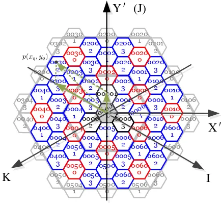
In this conversion, we introduce a three-axis coordinate system
IJK
O
as shown in Figure 5. The origin ofIJK
O
is consistent with O0 X0Y0, and J-axis is the same as Y0-axis. The included angles of the three axes in the positive direction are all
120
±, which divides the plane into six quadrants.The basic idea of this conversion is that given a point
P (B ;L )
on the sphere, compute the 2D Cartesian coordinate p(xp;yp) on theO
X Y
of a single triangular face according to the location parameters of the regular icosahedron and forward solution of Snyder Projection. Then, in terms of the relationship of the triangular faces, face tile and vertex tile, converse p(xp;yp) to p(xq;yq) on the correspongding tileO0 X 0Y0 this point belongs to. In
IJK
O
, using the parallelogram law, project p(xq;yq) to the 2 axes wich are more closer to it and obtain two component code 1 and 2 in the two axes. Finally, add 1 and 2 in terms of rule of code addition and get the location code wherep
is located.The result (Ai; ) or (Vi; )comprises the tile and location code associated with
p
.0030
Figure 5. Conversion from geographic coordinates and location codes
N
fn 1g=
8
>
<
>
:
3 D
B in(k)
2 I
1 D
B in(k)
2 J
2 D
B in(k)
2 K
wherek
denotes the position of lattice at the axis andD
B in(k)
represents the binary number ofk
. Although the first digit doesn’t match the rule of binary system, its relation withk
is easy to obtain as well. Finally, in terms of code addition, the location code of the cellp
is inside is given by= 1 2
4.2 Conversion from location codes to geographic
coordinates
The conversion from location codes to geographic coordinates is easier. For the icosahedral code structure, the same code will exist in different tiles, hence apart from the location code, the index of the face tile or vertex tile is needed to be given as well. Given (Ai; ) or (Vi; ), the detailed steps are as the following:
1. Compute the complex number representation of the
location code .
According to Section 2, the lattice is number of a special form on the complex plane and the form of location code is just another efficient representation for it. Location code and complex number of the lattice can transform each other. Let the level of grid be n, = e1e2 en, ²en = 0| {z }0
n 1
;n > 2;
e 2 f0 ;1 ;2 ;3 g, the complex number of denoted C ( ) is that
C ( ) = C (e1e2 en)
= C (e1) + C (²e2
1 ) + C (²
e2
2 ) + C (²enn)
= 2n!0e1+ 2n 1!e2 + + 2!en
= 2n!0e1+
n X
i= 2
2n i+ 1!ei
here the real part and imaginary part of C ( ) are corresponding to (xq;yq) in the coordinate system of tiles .
2. Translate and rotate (xq;yq) into p(xp;yp) in the in the coordinate system of triangular faces.
3. Via the inverse computation of Snyder Equal-area Map projection, obtain the resulitinf (B ;L ). The detailed process of inver computation can refer to Snyder (1992) and Ben et al. (2006).
5. EXPERIMENTS AND ANALYSIS
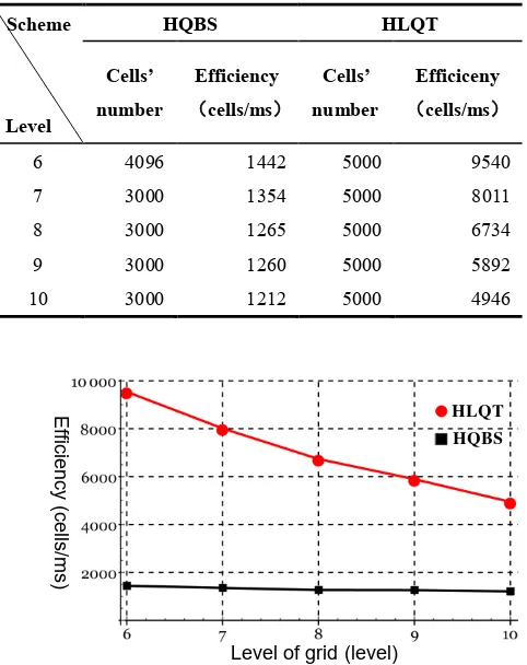
To verify the efficiency of the algorithm, we test the efficiency of code addition for the HLQT scheme and compare it with HQBS in that both the 2 shcemes use A4H and Snyder projection and the important factor influencing efficiency is the effiency of code operation. We adopt Visual C++ 2012 ad the development tool, compile the two algorithms into release versions and operate on the same compatible PC (Configuration: Intel Core i5-4590 [email protected] ,8G RAM, KingSton 120GB SSD; Operating System:Win 7 X64 Ultimate SP1; ). The result and the correlation curve of efficiency are shown in Table 3 and Figure 6 respectively.
We can see from Figure 6 that the efficiency of code addition of HLQT is obviously higher than HQBS and about 5 times the efficiency of code addition of HQBS.
Table 2. Statistical Results of computaional efficency about the two codes schemes
Scheme
Level
HQBS HLQT
Cells’ number
Efficiency δcells/msε
Cells’ number
Efficiceny δcells/msε
6 4096 1442 5000 9540
7 3000 1354 5000 8011
8 3000 1265 5000 6734
9 3000 1260 5000 5892
10 3000 1212 5000 4946
HQBS HLQT
Level of grid (level)
Efficien
cy
(cell
s/ms
)
6. CONCLUSIONS
This paper designs an encoding scheme named HLQT for the planar hexagonal aperture 4 grid system. Via the struture ‘face tile’ and ‘vertec tile’, we map this scheme onto the surface of the regular icosahedron and based on this, purpose a new algorithm of conversion between geographic coordinates and location codes. By contrast experiments, the superiority of HLQT in efficiency is verified.Moreover, this paper just realize the conversion between geographic coordinates and location codes. In order to realize geospatial data with different forms entering and getting out of DGGS, there is still lot of work needed to be done.
ACKNOWLEDGEMENTS
Portions of this research were supported by National Natural Science Foudation of China (Grant NO. 41671410) and by Special Financial Grant from the China Postdoctoral Science Foundation (Grant NO. 2013T60161). The research has not been subjected to the Committee of National Natural Science Foundation or the Committee of Postdoctoral Science Foundation’s peer and administrative review and, hence, does not necessarily reflect the views of them.
REFERENCES
Ben J. 2005. A Study of the Theory and Algorithm of Discrete Global Grid Data Model for Geospatial Information
Management. Dissertation Submitted to PLA Information Engineering University for the Degree of Doctor of
Engineering. Zhengzhou: Information Engineering University
Ben J, Tong X, Zhang Y, etc. 2006. Snyder Equal-area Map Projection for Polyhedral Globes[J]. Geomatics and Information Science of Wuhan University, 31(10):900-903
Ben J, Tong X, Zhang Y, etc. 2007. A Generation Algorithm for a New Spherical Equal-Area Hexagonal Grid System. Acta Geodaetica et Cartographica Sinica, 36(5):187-191
Ben J, Tong X, Wang L, etc. 2010. Key Technologies of Geospatial Data Management Based on Discrete Global Grid System. Journal of Geomatics Science and Technology, 27(5):382-386
Ben J, Tong X, Yuan C. 2011. Indexing Schema of the Aperture 4 Hexagonal Discrete Global Grid System. Acta Geodaetica et Cartographica Sinica,40(6):785-789
Ben J, Tong X, Zhou C, etc. 2015a. The Algorithm of Generating Hexagonal Discrete Grid Systems Based on the Octahedron. Journal of Geo-Information Science.
17(7):789-797
Ben J, Zhou C, Tong X, etc. 2015b. Design of Multi-level Grid System for Integrated Scientific Investigation of Resources and Environment. Journal of Geo-Information Science,
17(7):765-773
Peterson 2006. Close-Packed Uniformly Adjacent, Multi-resolution Overlapping Spatial Data Ordering.
Sahr K, White D, Kimerling J. 2003. Geodesic Discrete Global Grid Systems. Cartography and Geographic Information Science, 30(2): 121-134
Sahr K. 2011. Hexagonal Discrete Global Grid Systems for Geospatial Computing. Archives of Photogrammetry, Cartography and Remote Sensing, 22: 363-376
Sahr K. 2005. Discrete Global Grid Systems: A New Class of Geospatial Data Structures. Ashland: University of Oregon
Sahr K. 2008. Location Coding on Icosahedral Aperture 3 Hexagon Discrete Global Grids. Computers, Environment and Urban Systems, 32(3): 174-187
Snyder J P. An equal-area map projection for polyhedral globes[J]. Cartographica, 1992, 29(1): 10-21
Tong X. 2010. The Principle and Methods of Discrete Global Grid Systems for Geospatial Information Subdivision Organization. A Dissertation Submitted to PLA Information Engineering University for the Degree of Doctor of
Engineering. Zhengzhou: Information Engineering University
Tong X, Ben J, Wan Y, etc. 2013. Efficient Encoding and Spatial Operation Scheme for Aperture 4 Hexagonal Discrete Global Grid System. International Journal of Geographical Information Science, 27(5): 898-921
Vince A, Zheng, X. 2009. Arithmetic and Fourier Transform for the PYXIS Multi-resolution Digital Earth Model. International Journal of Digital Earth, 2(1): 59-79
Vince A, 2006a. Indexing the aperture 3 hexagonal discrete global grid. Journal of Visual Communication & Image Representation, 17: 1227-1236