TWO METHODS FOR REMOTE ESTIMATION OF COMPLETE URBAN SURFACE
TEMPERATURE
Lu Jianga, Wenfeng Zhana,b,
*
, Zhaoxu Zoua aJiangsu Provincial Key Laboratory of Geographic Information Science and Technology, International Institute for Earth System Science, Nanjing University, Nanjing, Jiangsu 210046, China – [email protected]; [email protected] b
Jiangsu Center for Collaborative Innovation in Geographical Information Resource Development and Application, Nanjing, 210023, China – [email protected]
Commission IV, WG IV/3
KEY WORDS: Urban surface; Thermal anisotropy; surface temperature; complete urban surface temperature; Semi-hemispherical temperature; kernel-driven model.
ABSTRACT:
Complete urban surface temperature (TC) is a key parameter for evaluating the energy exchange between the urban surface and
atmosphere. At the present stage, the estimation of TC still needs detailed 3D structure information of the urban surface, however, it is
often difficult to obtain the geometric structure and composition of the corresponding temperature of urban surface, so that there is still lack of concise and efficient method for estimating the TC by remote sensing. Based on the four typical urban surface scale models,
combined with the Envi-met model, thermal radiant directionality forward modeling and kernel model, we analyzed a complete day and night cycle hourly component temperature and radiation temperature in each direction of two seasons of summer and winter, and calculated hemispherical integral temperature and TC. The conclusion is obtained by examining the relationship of directional radiation
temperature, hemispherical integral temperature and TC: (1) There is an optimal angle of radiation temperature approaching the TC in a
single observation direction when viewing zenith angle is 45 ~ 60 °, the viewing azimuth near the vertical surface of the sun main plane, the average absolute difference is about 1.1 K in the daytime. (2) There are several (3~5 times) directional temperatures of different view angle, under the situation of using the thermal radiation directionality kernel model can more accurately calculate the hemispherical integral temperature close to TC, the mean absolute error is about 1.0 K in the daytime. This study proposed simple and
effective strategies for estimating TC by remote sensing, which are expected to improve the quantitative level of remote sensing of
urban thermal environment.
1 INTRODUCTION
Urban surface temperature (UST) is a variable crucial to the estimation of surface radiation and energy budgets, and it therefore plays an important role in the investigation of urban climate and environment (Voogt & Oke, 2003). Thermal infrared remote sensing (TIR) provides an indispensable way to obtain USTs at a large scale (Li et al., 2013). Nevertheless, this technique usually detects the surface thermal radiation (or temperature) in a certain or very few observation angles, i.e., T(θ, φ), where θ and φ are the viewing zenith and azimuth angles, respectively, while urban surfaces demonstrates significant thermal anisotropy during both the daytime and nighttime (Lagouarde et al., 2010; Lagouarde et al., 2012). It is thus rather difficult for the TIR technique to obtain a UST adequately descriptive to represent the true surface thermal status.
The estimation of the representative USTs requires the deep understanding of urban thermal anisotropy (UTA). Both field and airborne experiments as well as computer modelling have been used to understand the regime of UTA (Soux et al., 2004; Yu et al., 2006; Voogt, 2008; Lagouarde et al., 2010, 2012; Zhan et al., 2012; Ma et al., 2013; Allen et al., 2017). Their results show that, when compared with the natural surfaces dominated
* Corresponding author
primarily by vegetation, urban surfaces exhibit a more noteworthy hot-spot effect: The UTA intensity at noon can be as high as 10.0 K or more in a clear sky, but it decreases rapidly after sunset (Voogt, 2008; Lagouarde et al., 2010; Zhan et al., 2012). In view of the higher structural complexity of urban surfaces, kernel-driven models that are able to reconstruct radiation temperatures at all directions within the upper hemisphere using only several directional radiation temperatures (DRTs) have also been developed recently (Vinnikov et al., 2012; Sun et al., 2015; Duffour et al., 2016). These kernel-driven models are capable of modifying the DTRs into nadir temperatures and further have the potential to acquire a UST sufficiently representative of the urban thermal status.
calculated directly according to its standard definition by combining detailed field measurements on component surface temperatures and fractions (Voogt & Oke, 1997; Voogt, 2000). Their results confirmed that there was a large difference between Tc and the nadir temperature, and preliminary analysis illustrated that the DRTs with more shadowed component areas contained in the observational field of view (FOV) would be closer to Tc. Further research indicated that the hemispherical radiation temperatures (HRTs) measured by pyrgeometers are better for approaching Tc (Roberts et al., 2009; Adderley et al., 2015).
Although preliminary progress has been made on the estimation of Tc, currently the remote estimation of Tc from airborne or spaceborne observations without the assistance of ground-based measurements remains challenging, mostly because of the difficulty to accurately quantify the component temperatures and fractions for complex urban surfaces from a remote sensing perspective. For the remote estimation of Tc, issues need to be solved in the following two aspects: (1) is there an optimal remote sensing observation angle (view) that is close to Tc in a single observation angle? (2) In the case of radiation temperatures with several viewing angles, can the hemisphere integral temperature reconstructed by the thermal infrared kernel model, be used to approximate the Tc?
To answer these two questions, based on the simplified scale model of typical urban surface with different height width ratio (Building-Height-to-Spacing-Width ratios, H/W), this paper calculates T(θ, φ) in each viewing angle of urban surface by computer simulation, seeks for the optimal viewing angles approaching Tc, and further explores the possibility of directly approaching Tc by kernel model with several directional radiation temperatures. In order to obtain the accurate method for the estimation of Tc by remote sensing under various observation scenarios, this paper supports the improvement of
the quantization level of urban environment remote sensing.
2 DATA AND METHODS
2.1 Scale model for typical urban surfaces
The geometric structure of urban surface is complex, and the building density, building height and street width have a direct impact on urban surface temperature.
In order to include all kinds of typical urban surface types, this paper puts forward the local climate zoning (LCZ) according to Stewart and Oke (2012), 3ds-Max software is used to design four kinds of physical scale models of three dimensional structure of typical urban surface called typical urban surface(TUS)(Fig.1)
which with different building density (dense or sparse distribution), building height (high, low or mixed layer):TUS01 is a densely distributed group of tall buildings (such as a city center, a business district, etc.); TUS02 is sparsely distributed low rise buildings (such as urban light industrial or residential areas); TUS03 is a sparse distribution of high and low buildings (e.g. City, commercial, residential, mixed, etc.); TUS04 is a large sparse building with sparse distribution (such as large workshop type industrial district). The surface geometry and other related parameters of the four physical scale models are shown in Table 1.
2.2 Simulation of component temperature
Urban microclimate software Envi–met, one of the mainstream of urban environment and microclimate simulation software, its simulation of the surface temperature effect is good (Chow et al., 2011; Huang et al., 2015), it will mainly use Envi - met simulate urban surface temperature (components temperature). Compared
.
Fig.1. Scale models of four typical urban surfaces (TUS).
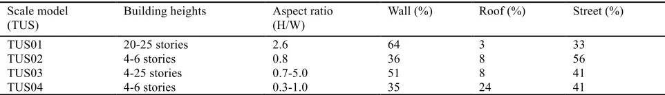
Table.1. The geometric structure parameter information of four types of urban underlying surface model includes the building type, building height and street width ratio (H/W), and the surface area of the ground surface, which accounts for the weight of the whole
surface. Scale model
(TUS)
Building heights Aspect ratio (H/W)
Wall (%) Roof (%) Street (%)
TUS01 20-25 stories 2.6 64 3 33
TUS02 4-6 stories 0.8 36 8 56
TUS03 4-25 stories 0.7-5.0 51 8 41
TUS04 4-6 stories 0.3-1.0 35 24 41
to the spring and autumn season, urban underlying surface thermal radiation directivity characteristics more typical representative in summer and winter (Lagouarde et al. 2010), and the main consideration two seasons (summer and winter) in this paper. On the basis of the foregoing city of building physical scale model, we simulate the surface temperature of Nanjing, China (118.54 °E, 31.56 °N) in four types of physical scale
model in a whole day and night cycle in summer and winter.
mesh. The grid resolution were dx=4 m, dy=4 m and dz=6 m (dx and dy, horizontal resolution of X, Y; dz, vertical resolution of Z). (2) The simulation start time is set in July 29, 2015 (winter time is January 15, 2016) 06:00, and the simulation lasts 24 hours. (3) Meteorological forcing data using the site measured value, the initial air temperature is 26 °C (06:00 measured average), with the prevailing southwest wind (wind direction azimuth angle is 240°), 10 m height wind speed was 1.0 m/s (measured average value), the relative humidity is 90% (measured).
Under the influence of solar radiation, the urban surface temperature in daytime and shadow is different greatly, and the trend of the surface temperature of different building faces is different. In order to better carry out radiation forward simulation heat according to the statistical characteristics of the surface temperature of the building facade in different city, the city is divided into surface light / shadow under the ground, the east wall, west wall, south wall, north wall, roof (a total of 12 kinds of component types (Zhan et al. 2012). The surface temperatures of the 12 types of components are calculated directly by the mesh surface temperature of the Envi-met simulations.
2.3 Forward simulation of directional radiation
temperature
On the basis of the aforementioned urban surface physical scale models and component temperature as input, in this paper, the directional radiation temperature T(θ, φ) of the urban surface in the upper hemisphere (the observation position of sensor, zenith angle is 0~90°(interval set to 10°), and azimuth is 0~360°(interval is set 30°)) is calculated directly by using the CoMSTIR (Computer Model to Simulate the Thermal Infrared Radiation of 3-D urban targets) model of urban surface thermal radiation. The model of CoMSTIR has a more rigorous physical basis, and its simulation result precision (RMSE) reaches 0.7 K (Ma et al., 2013). The geographical location information (longitude and latitude), observation time, sensor space position parameters are required, when T(θ, φ) is simulated by CoMSTIR.
2.4 Simulation of directional radiation temperature by
kernel model
By means of surface thermal radiation direction of nuclear driven simulation model proposed by Vinnikov et al. (2012) (hereinafter referred to as Vinnikov model), on the basis of only a few known T(θ, φ), the T'(θ, φ) in all directions of the upper hemisphere is reconstructed. The semi-empirical statistical model——Vinnikov model ponders the surface temperature changing with angle under the "Sensor - Target - Sun "three different relative position relation, has higher accuracy (RMSE value less than 1 K), is suitable for the simulation of city surface thermal anisotropy (Sun et al., 2015; Duffour et al., 2016).The model can be expressed by the following simple equation:
[
]
0
( , ,
i)
1
( )
( , ,
i)
T
θ θ
Δ
ϕ
=
T
⋅
+
A
⋅Φ
θ
+
D
⋅ Ψ
θ θ
Δ
ϕ
1where, θ、θi与∆φ are sensor viewing zenith angle, solar zenith
angle and sun-sensor relative azimuth angle; T0 is nadir radiance temperature; A and D are coefficients of kernel driven model; Φ(·) and Ψ(·) are the "the emissivity kernel" and "the solar kernel".
2.5 Calculation of integral temperature and complete
surface temperature
Hemispherical Angle Integral temperature (TH) for the specific direction of solid angle range Ω radiation temperature T(θ, φ) integral, its computation formula is as follows:
weighted sum, of the product of specific calculate formula is as follows (Voogt & Oke, 1997): components are set in section 2.2).
2.6 Remote sensing estimation/approximation strategy of
Tc
2.6.1 Single direction observation
In order to obtain the T(θ, φ) of optimal angle which close to Tc under the single direction observation by remote sensing, we will use CoMSTIR to simulate four typical urban surfaces (TUS01~TUS04), 24 day time intraday (hourly), 2 typical seasons (summer and winter),and get a total of 192 polarization diagrams of T(θ, φ) (i.e. Zenith angle range of 0~90°; the azimuth angle is in the range of 0~360°). The T(θ, φ)which is closest to Tc in the mean sense, is comprehensively investigated.
2.6.2 Multi-directional observations
In order to obtain a remote sensing estimation / approach Tc method in a multi direction observation scenario, the TH(Ω), which is closest to Tc in the mean sense, is evaluated in a comprehensive manner. The TH(Ω) including TH(0~0°, 0~360°) (i.e. nadir radiation temperature, the follow-up will be directly marked as T0), TH(0~30°, 0~360°) (marked as Th30), TH(0~60°, 0~360°) (marked as Th60), TH(0~90°, 0~360°) (i.e. hemisphere integral temperature, marked as Th90), and Toa (optimal view angle direction radiation temperature).In addition, 4 observation angles with more uniform distribution are selected, including (20°, 30°), (40°, 120°), (50°, 330°) and (60°, 240°). Based on the T(θ, φ) at these angles, the radiation temperature T'(θ, φ) in each direction is reconstructed by the Vinnikov model(in section 2.4), and the capability of approximating the Tc with the optimal hemispherical angle integral temperature calculated on the basis of T'(θ, φ) is investigated.
3 RESULTS
3.1 Comparison of T(θ, φ) and Tc
"effect (the azimuth of "hot spot" is close to sun's) is obvious. At 13:00 of summer, corresponding to the zenith angle of "hot spot" is about 30°(Fig.2.b), and the zenith angle of "hot spot" of the rest of 09:00 and 17:00 of summer and three-time of winter is close to 90°respectively, this may because of at summer noon (13:00) of the solar zenith angle is much smaller than others shown in the figure.
As shown in fig.2, the value of Tc is between the maximum and minimum values of T(θ, φ), and is relatively closer to the minimum value of T(θ, φ). The contour line of Tc occasionally approximates the nadir radiation temperature T0, for example,
the difference is only 1.0 K at 09:00 in summer. However, there may also be significant differences between T0 and Tc, and T0 can not simply replace Tc. The physical scale model of LCZ03 as an example, at 13:00 of summer and 09:00 of winter, the difference of Tc and T0 can be up to 4.4 and 4 K. The simulation results for all physical scale models and all day time further show that the range of ∆T is up to 6.0 K (LCZ01; at 17:00 of summer), the average absolute value of approximately 2.0 K (2.04 K). The above results preliminarily illustrate that the nadir direction is not the best observation angle by remote sensing for the direct acquisition of Tc in the case of only a single observation direction.
Fig.2 The polar-DRT of daytime typical time of summer and winter over the scale model (TUS03) and contour of Tc (unit K). The black cross indicates the position of "hot spot", the "S" indicates the position of sun. And, (a), (b) and (c) are in summer, (d), (e) and
(f) are in winter, the zenith angle and azimuth range are 0~90° and 0~360° respectively.
3.2 Optimal angle of Tc under a single direction
As far as the single temperature polarization diagram is concerned, the zenith angle and azimuth angle of the contour of Tc can be considered as the best observation angle of approaching Tc. In order to find the optimal angle (sight) for all scale models and moments can approximate Tc, we integrate the contours of Tc in the polarization graph of T(θ, φ) of all scale models at a particular moment, and obtain the contour (the best viewing angle) set of approaching Tc( Fig.3).Considering the difference of the sun position between winter and summer, we rotate the solar main plane (temperature polarization diagram) corresponding to the winter to the position of the solar main plane in summer (S - S').
As seen from Fig.3, the contours of Tc converge closely in or around the elliptical dotted line in the figure, that is, the position indicated by the dotted circles are the optimal angle field approaching the Tc. For the different times in the daytime (Fig.3), the marked dotted circles are roughly located near the vertical plane of the solar main plane, that is, the azimuth angle of optimum observation is approximately equal to the solar azimuth ±90°, and the zenith angle of optimum observation is about 45~60°.TUS03 still as example, at 11:00, 13:00 and 15:00 in the summer, compare the temperature value of T(60, 180), T(60, 300) and T(60, 330) in (or near) dotted circle to Tc which the corresponding time, the difference |∆T| is only 0.49, 0.37 and 0.27 K, respectively(for the simulated temperature value by
section 2.6.2 of T'(60, 180), T'(60, 300) and T'(60, 330), the difference |∆T'| is 1.43、1.11 and 1.51 K, respectively). Much smaller than the difference between T0 and Tc (the mean value of the difference is 2.89 K at these three moments). This is possible because when the view azimuth in the solar principal plane vertical orientation, the sensor can be more evenly to get the sunlight and shadowed face of the urban surface at the same time, so that the observed T(θ, φ) can reflect more comprehensive information of Tc.
optimal observation of general urban surface condition, further polarization diagram of average absolute difference |∆T|mean between Tc and T(θ, φ) of all scenarios is obtained (Fig.4).
This polarization diagram(Fig.4) shows that if the value of a domain (view) is smaller, the field tends to be closer to the Tc. In the hemisphere space, the range of |∆T|mean is about 1.0~9.0 K. The value of |∆T|mean is larger where the solar principal plane direction (the azimuth including toward and inverse to the sun) with larger zenith view angle (up to 5.5 K or more, that is not suitable as a view of approaching Tc). In contrast, the value of |∆T|mean is relatively small (it is only 1.2 K or less) where the view in the solar principal plane vertical azimuth and zenith angle is approximately 45~60°, this view can become optimal view of approaching Tc, as the results shown in Fig.3. Voogt and Oke (1997) did ground and flight observation in typical urban surface (including light industrial area, downtown and
residential areas), the observation of the position of the sun are mostly in the East direction (08:00~10:00, that in the early morning) or the West direction (15:00~17:00, that in the late afternoon), and fixed viewing zenith angle at 45°, the research shows that the azimuth angle is close to the North (near vertical surface at this time when the azimuth is located in the main plane of the sun), T(θ, φ) can better approximate Tc. Although the structure and material of urban surface are different, the conclusion is similar to that of this study. The difference is that, due to the limitation of the cost of observation and conditions, Voogt and Oke (1997) demonstrated only the fixed viewing zenith angle is 45°, the viewing azimuth angle is located at the North direction is the best of the East, West, South and North direction. Through the complete simulation of the hemisphere space in the whole urban surface heat radiation, this paper gives the optimal observation under various scenarios of average.
Fig.4 The polar-|∆T|mean of average absolute difference between Tc and T(θ, φ) (the sun azimuth is unified and rotated to the
south).
3.3 Comparison of TH(Ω) and Tc
The above is mainly given that the optimal observation field under the single observation direction T(θ, φ). In order to estimate Tc more accurately by remote sensing, this section focuses on how to use the integral temperature to get closer to the Tc with several T(θ, φ). This section selects the integral temperature mainly include Toa (integral interval is the optimal view) and Thx (integral interval is θ∈[0, x], φ∈[0, 360]). The comparison of TH(Ω) and Tc is shown in Fig.5.
Based on the daily variation of the difference between t TH(Ω) and Tc, the following conclusions are obtained: (1)On the integral temperature, due to the strong effect of solar radiation during the daytime, the difference between sunlit and shadow component temperature is large, so |Thx-Tc| is larger in the daytime, smaller at night, and the absolute difference is directly related to the value of the component temperature (or solar radiation).(2)The greater the range of the zenith angle integration [0, x], the closer the Thx is to Tc. In summer(Fig.5.a), for example, the average absolute difference |∆T|mean between Thx and Tc, with integral zenith angle increased from 0°, 30°, 60° and then increased to 90°, | the value of |∆T|mean from 1.33, 1.12, 0.84 K
Fig.5 Comparison of TH(Ω) and Tc. And, (a) and (b) indicate summer and winter, respectively. Tc is complete surface temperature, Thx is integral temperature of the azimuth angle is from 0 to 360° and the zenith angle is from 0 to x, Toa is integral temperature of optimal view area. The vertical axis on the left and right shows the temperature value of Tc and the absolute difference between Thx,
Toa and Tc, respectivel.
Fig.6 Comparison of Th based on kernel model and Tc. The Y-axis is the mean absolute difference |∆T| between hemisphere integral temperature and Tc, the circle represents the mean of |∆T| and the bound of 0.5 times standard deviation. The ∆Th is absolute difference |∆T| calculated from Th (calculated by the original T(θ, φ)) and Tc, The ∆Thv is absolute difference |∆T| calculated from Thv (calculated by T'(θ, φ) simulated by Vinnikov model) and Tc, the latter 1, 2, 3 and 4 represent 4 classes of TUS, respectively.
and then decreases to 0.44 K. In other words, hemisphere integral temperature Th90 can be the most accurate approximation of Tc, even in the summer, the lowest precision of 13:00, the difference between Th90 and Tc is only 1.48 K, and this accuracy is quite to most satellite surface temperature product. (3)The integral temperature Toa which in a relatively narrow optimal view is slightly worse than Th90 in approaching Tc, but slightly
better than Th60. In the daytime, the average absolute difference between the three integral temperature (Toa, Th90 and Th60) and Tc is 1.11, 0.66 and 1.26 K, respectively (Fig.5).
be accurately approximated Tc (Roberts & Voogt, 2009). It is also shown that the integral temperature of a single narrow field of view (even the optimal observation horizon) is difficult to approximate the hemisphere integral temperature in terms of the ability to approach Tc. directionality model. In general, forward modeling requires detailed surface geometry and component temperature information (Voogt, 2008; Lagouarde et al., 2011; Zhan et al., 2012). It is conceivable that such detailed structure and temperature information are difficult to obtain in remote sensing of urban thermal environment. Only by considering the thermal infrared remote sensing observation in a few directions, the Th inversion can be carried out, and the estimation of Tc by remote sensing is feasible. In this section, we test the estimation of hemispheric integration temperature based on the kernel model (hereinafter referred to as Vinnikov model)developed by Vinnikov et al. (2012), and then estimate the approximation capability of the simulated hemisphere integration temperature to Tc. For this purpose, the T'(θ, φ) obtained from the section 2.6.2 is used to estimate the hemispheric integral temperature (Thv). Fig.6 shows the different types of TUS scenario, compares the difference value among Tc and Th calculated from original T(θ, φ) and Thv calculated from Vinnikov model, that is ∆Th and
∆Thv.
From the dimensions of the physical csale model, the difference between ∆Th and ∆Thv is 0.39 ~ 0.97 K in summer, in contrast, the difference is smaller in winter, that is only 0.24~0.53 K. From the perspective of different moments of the day, the average values of ∆Th and ∆Thv are 0.76 and 1.44 K in the summer daytime (07:00~17:00), 0.12 and 0.19 K in the summer night (19:00~05:00). In winter, the average values of ∆Th and
∆Thv are 0.50 and 0.63 K in daytime (09:00~17:00), 0.13 and 0.17 K at night (19:00~07:00). Accordingly, the following conclusions are drawn: (1) Overall, Th is closer to Tc than Thv.(2) The difference between ∆Th and ∆Thv in all night time of summer and winter and winter daytime is so small that can be ignored, the difference is about 0.70 K in the summer daytime. Although Thv is slightly worse than Th in the Tc approximation ability, methods provided in this paper are more accurate estimation of surface temperature. The process of land surface temperature inversion, influenced by the factors of emissivity, atmospheric effect, errors are inevitably introduced into the observation or simulation, several directional radiation temperature observations may introduce errors repeatedly, together with errors introduced during the simulation by kernel model, whether that estimation of Tc adopts a optimal angle observation is better. In fact, in satellite remote sensing observation, there are differences in solar positions at different times, it is difficult to
obtain Toa at any time. So, in practical remote sensing observation, Toa is used to represent Tc in the case of Toa can be obtained, or there are several (3~5) T(θ, φ), Tc is represented by the hemispherical integral temperature calculated by kernel model.
(2) At present, temperature inversion accuracy is low (about 2~3 K) by thermal infrared remote sensing in urban area, the approximation accuracy of Tc can reach 1.0 K in this paper , the relative accuracy on the angle dimension (accuracy of T(θ, φ) and Th approximation to Tc), there is essential difference to the surface temperature inversion accuracy. In the follow-up study, even if the temperature inversion accuracy of urban area is increasing continuously, the temperature characteristics of urban underlying surface can not be accurately described if the directional difference caused by viewing angle can not be solved. Two methods for estimating Tc provided in this paper are mainly to solve the problem of angle dimension, and are able to bring the observation direction error to a minimum, to get the most close to the real urban surface temperature in the present remote sensing surface temperature inversion accuracy.
(3)Due to the complex three-dimensional structure of urban surface, the more change of sunlit or shadowed component surface, and rapidly changing temperature, it is difficult to obtain the detailed surface temperature in field measurement, and the error of time scale is difficult to eliminate. The models used in this paper (including land surface temperature simulation - Envi-met, directional radiation temperature simulation - CoMSTIR, kernel model simulation - Vinnikov model) are all classic models, simulation accuracy has been widely recognized. In addition, compared with the field observation conducted over a few days, land surface temperature of only a few areas can be obtained. This paper provides more data to analyze, find out the law and solve the scientific problems.
4.2 Shortages and prospects
2017), sensible heat flux and air temperature in urban area in the follow-up research work.
5 CONCLUSIONS
Traditionally, accurate estimation of complete urban surface temperature requires detailed surface 3D structural information with component temperature data. In this paper, the optimal observation angle (sight) of Tc (directional radiation temperature T(θ, φ)) is studied under the condition of only one observation, as well as in scenario, with multiple observations using the thermal radiation directionality kernel model to simulate the possibility of Th close to Tc. The results show that: (1) in the case of only a single observation angle, in order to approach Tc, the optimal observation zenith angle of the sensor should be at 45~60°, and the observation azimuth should be near the vertical plane of the solar main plane. The quantitative calculation shows that the average absolute error of T(θ, φ) and Tc is only 1.11 K when the observation angle (sight) is in the optimal observation angle. (2) As a complete characterization of the thermal radiation characteristics of urban surfaces in all directions, the hemispheric integral temperature Th can be used instead of Tc, and its ability to approach Tc is superior to that of T(θ, φ) at the optimum observation angle. (3) In the case of multiple directional thermal infrared observations, the hemispheric integral temperature based on the kernel model can also be used to directly substitute for Tc. About remote estimation of complete urban surface temperature, this paper provides a simple, accurate strategy, which is expected to serve the city surface atmosphere energy balance estimation, so as to promote and support the level of quantitative remote sensing of city thermal environment improvement. In addition, this paper is expected to provide a reference for further satellite orbit design for urban thermal environment observation.
ACKNOWLEDGMENTS
This work is supported by the National Natural Science Foundation of China under Grants 41671420 and 41301360, and by the Key Research and Development Programs for Global Change and Adaptation under 2016YFA0600201. We are also grateful for the financial support provided by the DengFeng Program-B of Nanjing University.
REFERENCES
Adderley, C., Christen, A., & Voogt, J. A., 2015. The effect of
radiometer placement and view on inferred directional and
hemispheric radiometric temperatures of an urban canopy.
Atmospheric Measurement Techniques, 8(7), 2699-2714.
Allen, M. A., Voogt, J. A., & Christen, A., 2017. Towards a
continuous climatological assessment of urban surface heat
islands. In Urban Remote Sensing Event (JURSE), 2017 Joint (pp.
1-4). IEEE.
Chow, W. T., Pope, R. L., Martin, C. A., & Brazel, A. J., 2011.
Observing and modeling the nocturnal park cool island of an arid
city: horizontal and vertical impacts. Theoretical and Applied
Climatology, 103(1-2), 197-211.
Duffour, C., Lagouarde, J. P., & Roujean, J. L., 2016. A two
parameter model to simulate thermal infrared directional effects
for remote sensing applications. Remote Sensing of
Environment,186, 250-261.
Dyce, D. R., & Voogt, J. A., 2017. The influence of tree crowns
on urban thermal effective anisotropy. Urban Climate.
Fontanilles, G., Briottet, X., Fabre, S., Lefebvre, S., &
Vandenhaute, P. F., 2010. Aggregation process of optical
properties and temperature over heterogeneous surfaces in
infrared domain. Applied Optics,49(24), 4655-4669.
Fontanilles, G., Briottet, X., Fabre, S., Trémas, T., & Henry, P.
(2008, October). TITAN: a new infrared radiative transfer model
for the study of heterogeneous 3D surface. In SPIE Remote
Sensing (pp. 71070F-71070F). International Society for Optics
and Photonics.
Hénon, A., Mestayer, P. G., Groleau, D., & Voogt, J., 2011. High
resolution thermo-radiative modeling of an urban fragment in
Marseilles city center during the UBL-ESCOMPTE campaign.
Building and Environment,46(9), 1747-1764.
Hu, L., Monaghan, A., Voogt, J. A., & Barlage, M., 2016. A first
satellite-based observational assessment of urban thermal
anisotropy. Remote Sensing of Environment,181, 111-121.
Huang, H., Xie, W., & Sun, H., 2015. Simulating 3D urban
surface temperature distribution using ENVI-MET model: Case
study on a forest park. In Geoscience and Remote Sensing
Symposium (IGARSS), 2015 IEEE International (pp. 1642-1645).
IEEE.
Krayenhoff, E., & Voogt, J., 2016. Daytime thermal anisotropy
of urban neighbourhoods: morphological causation. Remote
Sensing,8(2), 108.
Lagouarde, J. P., & Irvine, M., 2008. Directional anisotropy in
thermal infrared measurements over Toulouse city centre during
the CAPITOUL measurement campaigns: first results.
Meteorology and Atmospheric Physics, 102(3), 173-185.
Lagouarde, J. P., Hénon, A., Kurz, B., Moreau, P., Irvine, M.,
Voogt, J., & Mestayer, P., 2010. Modelling daytime thermal
infrared directional anisotropy over Toulouse city centre.
Remote Sensing of Environment,114(1), 87-105.
Lagouarde, J. P., Hénon, A., Irvine, M., Voogt, J., Pigeon, G.,
Moreau, P., Masson, V.& Mestayer, P., 2012. Experimental
characterization and modelling of the nighttime directional
anisotropy of thermal infrared measurements over an urban area:
Case study of Toulouse (France). Remote Sensing of
Li, Z. L., Tang, B. H., Wu, H., Ren, H., Yan, G., Wan, Z., ... &
Sobrino, J. A., 2013. Satellite-derived land surface temperature:
Current status and perspectives. Remote Sensing of Environment,
131, 14-37.
Poglio, T., Mathieu-Marni, S., Ranchin, T., Savaria, E., & Wald,
L., 2006. OSIrIS: a physically based simulation tool to improve
training in thermal infrared remote sensing over urban areas at
high spatial resolution. Remote Sensing of Environment, 104(2),
238-246.
Ren, H., Yan, G., Chen, L., & Li, Z., 2011. Angular effect of
MODIS emissivity products and its application to the
split-window algorithm. ISPRS Journal of Photogrammetry and
Remote Sensing, 66(4), 498-507.
Roberts, S. M., & Voogt, J. A., 2009. Outdoor scale model
experiment to evaluate the complete urban surface temperature.
Eighth Symposium on the Urban Environment.
Stewart, I. D., & Oke, T. R., 2012. Local climate zones for urban
temperature studies. Bulletin of the American Meteorological
Society, 93(12), 1879-1900.
Soux, A., Voogt, J. A., & Oke, T. R., 2004. A Model to Calculate
what a Remote SensorSees' of an Urban Surface.
Boundary-layer meteorology,111(1), 109-132.
Vinnikov, K. Y., Yu, Y., Goldberg, M. D., Tarpley, D., Romanov,
P., Laszlo, I., & Chen, M., 2012. Angular anisotropy of satellite
observations of land surface temperature. Geophysical Research
Letters, 39(23).
Voogt, J. A., 2000. Image representations of complete urban
surface temperatures. Geocarto International, 15(3), 21-32.
Voogt, J. A., 2008. Assessment of an urban sensor view model
for thermal anisotropy. Remote Sensing of Environment, 112(2),
482-495.
Voogt, J. A., & Grimmond, C. S. B., 2000. Modeling surface
sensible heat flux using surface radiative temperatures in a
simple urban area. Journal of Applied Meteorology, 39(10),
1679-1699.
Voogt, J. A., & Oke, T. R., 1997. Complete urban surface
temperatures. Journal of Applied Meteorology, 36(9), 1117-1132.
Voogt, J. A., & Oke, T. R., 2003. Thermal remote sensing of
urban climates. Remote sensing of environment, 86(3), 370-384.
Zhan, W., Chen, Y., Voogt, J. A., Zhou, J., Wang, J., Ma, W., &
Liu, W., 2012. Assessment of thermal anisotropy on remote
estimation of urban thermal inertia. Remote Sensing of
Environment, 123(123), 12-24.
Zhao, L., Gu, X., Yu, T., Wan, W., & Li, J., 2012. Modeling
directional thermal radiance anisotropy for urban canopy. In
Geoscience and Remote Sensing Symposium (IGARSS), 2012
IEEE International (pp. 3102-3105). IEEE.
Ma, W., Chen Y. H., Zhan, W. F., & Zhou, J., 2013. Thermal
anisotropy model for simulated three dimensional urban targets.
Journal of Remote Sensing, 17(1), 62-76.
Sun, H., Chen Y. H., Zhan, W. F., Wang, M. J., & Ma, W., 2015.
A kernel model for urban surface thermal emissivity anisotropy
and its uncertainties. Journal of Infrared and Millimeter Waves,
34(1), 66-73.
Yu, T., Tian, Q. Y., Gu, X. F., Wang, J., Liu Q., & Yan, G. J.,
2006. Modelling directional brightness temperature over a
simple typical structure of urban areas. Journal of Remote