THE EFFECT OF DECOMPOSITION METHOD AS DATA
PREPROCESSING ON NEURAL NETWORKS MODEL FOR
FORECASTING TREND AND SEASONAL TIME SERIES
Suhartono
Statistics Department, Institut Teknologi Sepuluh Nopember, Surabaya, Indonesia Email: [email protected]; [email protected]
Subanar
Mathematics Department, Universitas Gadjah Mada, Yogyakarta, Indonesia Email: [email protected]
ABSTRACT
Recently, one of the central topics for the neural networks (NN) community is the issue of data preprocessing on the use of NN. In this paper, we will investigate this topic particularly on the effect of Decomposition method as data processing and the use of NN for modeling effectively time series with both trend and seasonal patterns. Limited empirical studies on seasonal time series forecasting with neural networks show that some find neural networks are able to model seasonality directly and prior deseasonalization is not necessary, and others conclude just the opposite. In this research, we study particularly on the effectiveness of data preprocessing, including detrending and deseasonalization by applying Decomposition method on NN modeling and forecasting performance. We use two kinds of data, simulation and real data. Simulation data are examined on multiplicative of trend and seasonality patterns. The results are compared to those obtained from the classical time series model. Our result shows that a combination of detrending and deseasonalization by applying Decomposition method is the effective data preprocessing on the use of NN for forecasting trend and seasonal time series.
Keywords: decomposition, data preprocessing, neural networks, trend, seasonality, time series, forecasting.
1. INTRODUCTION
Many business and economic time series are non-stationary time series that contain trend and seasonal variations. The trend is the long-term component that represents the growth or decline in the time series over an extended period of time. Seasonality is a periodic and recurrent pattern caused by factors such as weather, holidays, or repeating promotions. Accurate forecasting of trend and seasonal time series is very important for effective decisions in retail, marketing, production, inventory control, personnel, and many other business sectors (Makridakis and Wheelwright, 1987). Thus, how to model and forecast trend and seasonal time series has long been a major research topic that has significant practical implications.
The aim of this paper is to develop new hybrid model by combining decomposition method as data preprocessing and NN model for forecasting trend and seasonal time series. The results are compared to ARIMA models.
2. MODELING TREND AND SEASONAL TIME SERIES
Modeling trend and seasonal time series has been one of the main research endeavors for decades. In the early 1920s, the decomposition model along with seasonal adjustment was the major research focus due to Persons (1919, 1923) work on decomposing a seasonal time series. Holt (1957) and Winters (1960) developed method for forecasting trend and seasonal time series based on the weighted exponential smoothing. Among them, the work by Box and Jenkins (1976) on the seasonal ARIMA model has had a major impact on the practical applications to seasonal time series modeling. This model has performed well in many real world applications and is still one of the most widely used seasonal forecasting methods. More recently, NN have been widely used as a powerful alternative to traditional time series modeling (see e.g. Hansen and Nelson ,2003; Nelson et al. ,1999; also Zhang et al. ,1998). While their ability to model complex functional patterns in the data has been tested, their capability for modeling seasonal time series is not systematically investigated.
In this section, we will give a brief review of these forecasting models, particularly seasonal ARIMA, decomposition method and NN model.
2.1 Seasonal ARIMA Model
The seasonal ARIMA model belongs to a family of flexible linear time series models that can be used to model many different types of seasonal as well as nonseasonal time series. The seasonal ARIMA model can be expressed as (see e.g. Box et al. ,1994; Cryer ,1986 and Wei ,1990):
t S Q q
t D S d
S P
p
B
B
B
B
y
θ
B
B
ε
φ
(
)
Φ
(
)(
1
−
)
(
1
−
)
=
(
)
Θ
(
)
, (1)where S is the seasonal length, B is the back shift operator and
ε
t is a sequence of white noises with zero mean and constant variance. Box and Jenkins (1976) proposed a set of effective model building strategies for seasonal ARIMA based on the autocorrelation structures in a time series.2.2 Decomposition Method
The multiplicative decomposition model has been found to be useful when modeling time series that display increasing or decreasing seasonal variation (Bowerman and O’Connel, 1993; chapter 7). The key assumption inherent in this model is that seasonality can be separated from other components of the series. The multiplicative decomposition model is
y
t=
T
t×
S
t×
C
t×
I
t (2)where
t
y
= the observed value of the time series in time periodt
t
T
= the trend component in time period tt
S
= the seasonal component in time period tt
C
= the cyclical component in time period tt
2.3 Neural Networks Model
Neural networks (NN) are a class of flexible nonlinear models that can discover patterns adaptively from the data. Theoretically, it has been shown that given an appropriate number of nonlinear processing units, NN can learn from experience and estimates any complex functional relationship with high accuracy. Empirically, numerous successful applications have established their role for pattern recognition and time series forecasting.
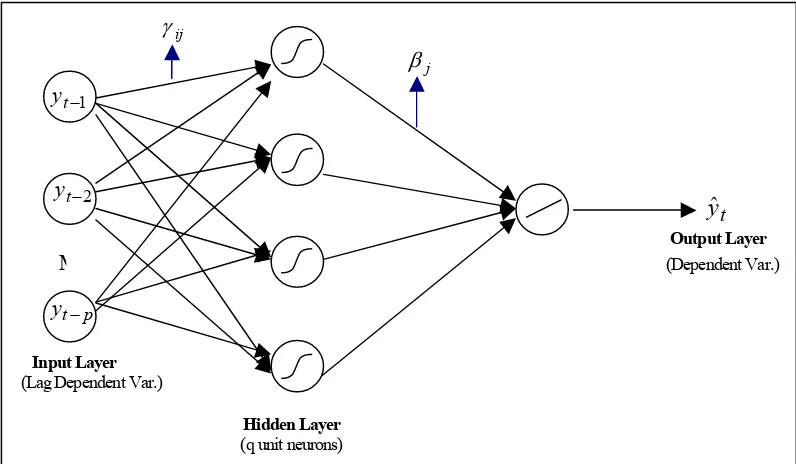
Feedforward Neural Networks (FFNN) is the most popular NN models for time series forecasting applications. Figure 1 shows a typical three-layer FFNN used for forecasting purposes. The input nodes are the previous lagged observations, while the output provides the forecast for the future values. Hidden nodes with appropriate nonlinear transfer functions are used to process the information received by the input nodes.
The model of FFNN in Figure 1 can be written as function such as the logistic:
indicates a linear transfer function is employed in the output node.
Functionally, the FFNN expressed in equation (3) is equivalent to a nonlinear AR model. This simple structure of the network model has been shown to be capable of approximating arbitrary function (see e.g. Cybenko, 1989; Hornik et al., 1989a, 1989b; and White, 1990). However, few practical guidelines exist for building a FFNN for a time series, particularly the specification of FFNN architecture in terms of the number of input and hidden nodes is not an easy task.
3. RESEARCH METHODOLOGY
The purpose of this research is to provide empirical evidence on the comparative study of many data preprocessing method in NN model for forecasting trend and seasonal time series. The major research questions we investigate is:
Does data preprocessing has a great impact on the accuracy of NN model for forecasting trend and seasonal time series?
Which data preprocessing is the most effective on NN model for forecasting model for trend and seasonal time series?
We conduct empirical study with simulation and real data, the international airline passenger data, to address these questions. This real data has been analyzed by many researchers; see for example Nam and Schaefer (1995), Hill et al. (1996), Faraway and Chatfield (1998), Atok and Suhartono (2000), Suhartono et al. (2005a, 2005b). This data also has become one of two data to be competed in Neural Network Forecasting Competition on June 2005 (see www.neural-forecasting.com).
3.1 Data
The simulation and real data contain 144 month observations. The first 120 data observations are used for model selection and parameter estimation (training data in term of NN model) and the last 24 points are reserved as the test for forecasting evaluation and comparison (testing data). Figure 2 plots representative time series of these data. It is clear that the series has an upward trend together with seasonal variations.
3.2 Research Design
Three types of data preprocessing based on the decomposition method are applied and compare to the airline data. Those are detrend, deseasonal, and combination detrend-deseasonal. All of these data preprocessing are implemented by using MINITAB software.
To determine the best hybrid model, that is combination data preprocessing based on the decomposition method and NN model, an experiment is conducted with the basic cross validation method. The available training data is used to estimate the weights for any specific model architecture. The testing set is the used to select the best model among all models considered. In this study, the number of hidden nodes varies from 1 to 10 with an increment of 1. The lags of 1, 12 and 13 are included due to the results of Faraway and Chatfield (1998), Atok and Suhartono (2000), and Suhartono et al. (2005a).
transform detrend, deseasonal, and combination detrend-deseasonal data to N(0,1) scale. The performance of in-sample fit (training data) and out-sample forecast (testing data) is judged by the commonly used error measures, the mean squared error (MSE) and ratio MSE to ARIMA model.
Figure 2. Time series plot of simulation and real data
4. EMPIRICAL RESULTS
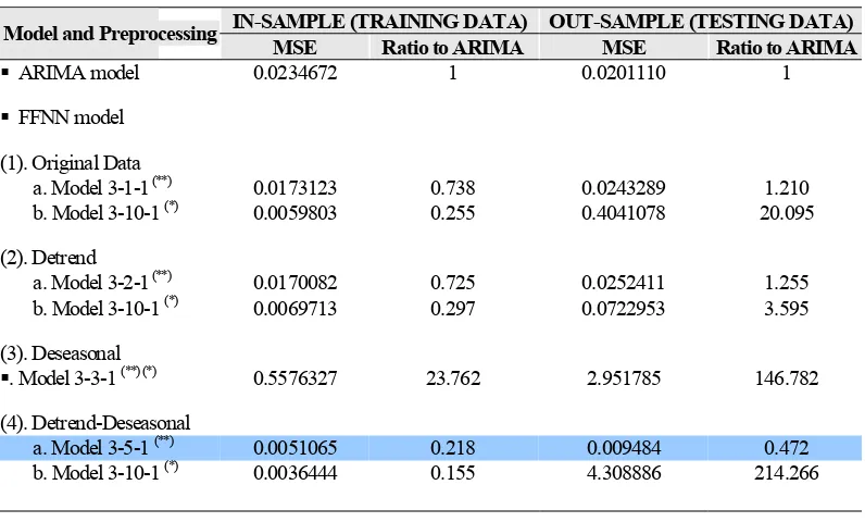
Table 1 summarizes the result of the impact of some data preprocessing on NN forecasting and report performance measures across training and testing samples for the simulation data. Numbers greater than one on column ratio indicates poorer forecast performance compare to the ARIMA models, and vice versa for numbers less than one.
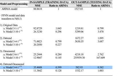
The results of the impact of some data preprocessing on NN forecasting and report performance measures across training and testing samples for the airline data are summarized in Table 2.
Testing data
Training data
Testing data
Training data
Simulation data
Several observations can be made from Table 1 and 2. First, detrend as data processing does yield poorer result than the original data or ARIMA. It can be clearly seen from Table 1 and 2 that the ratio MSE at testing samples for NN are greater than 1. Second, deseasonal as data processing gives the worst result than other data preprocessing and also compared to ARIMA. We can observe that the best model in testing samples by using deseasonal as data preprocessing yield the greatest ratio MSE compared to the results of the original data or the ratio of detrend as data preprocessing. Third, the combination detrend-deseasonal as data preprocessing yields the best result for forecasting the airline data. It can be shown by the least ratio of MSE at testing data.
Table 1. The result of the comparison between preprocessing data for FFNN and ARIMA models, both in training and testing data, for the simulation data.
IN-SAMPLE (TRAINING DATA) OUT-SAMPLE (TESTING DATA) Model and Preprocessing
: the best model in training data (in-sample forecast)
(**)
: the best model in testing data (out-sample forecast)
Table 2. The result of the comparison between preprocessing data for FFNN and ARIMA models, both in training and testing data, for the airline passenger data.
IN-SAMPLE (TRAINING DATA) OUT-SAMPLE (TESTING DATA) Model and Preprocessing
: the best model in training data (in-sample forecast)
(**)
: the best model in testing data (out-sample forecast)
5. CONCLUSIONS
Based on the results we can conclude that the combination detrend-deseasonal (based on the decomposition method) as data preprocessing in FFNN yields a great impact on the increasing accuracy of forecasting trend and seasonal time series. Our result also shows that the best model in training data tends to yield overfitting on testing. This condition give a chance to do further research by implementing some NN model selection methods in order for the model selection process becomes efficient.
REFERENCES
Atok, R.M. and Suhartono, 2000. Comparison between Neural Networks, ARIMA Box-Jenkins and Exponential Smoothing Methods for Time Series Forecasting, Research Report, Lemlit: Institut Teknologi Sepuluh Nopember.
Box, G.E.P. and G.M. Jenkins, 1976. Time Series Analysis: Forecasting and Control, San Fransisco: Holden-Day, Revised edn.
Bowerman, B.L. and R.T. O’Connel, 1993. Forecasting and Time Series: An Applied Approach,
3rd ed, Belmont, California: Duxbury Press.
Cryer, J.D., 1986. Time Series Analysis, Boston: PWS-KENT Publishing Co.
Cybenko, G., 1989. “Approximation by superpositions of a sigmoidal function”, Mathematics of Control, Signals and Systems, 2, 304–314.
Faraway, J. and C. Chatfield, 1998. “Time series forecasting with neural network: a comparative study using the airline data”, Applied Statistics, 47, 231–250.
Fildes, R. and S. Makridakis, 1995. “The impact of empirical accuracy studies on time series analysis and forecasting”, International Statistical Review, 63 (3), pp. 289–308.
Hanke, J.E. and A.G. Reitsch, 1995. Business Forecasting, Prentice Hall, Englewood Cliffs, NJ.
Hansen, J.V. and R.D. Nelson, 2003. “Forecasting and recombining time-series components by using neural networks”, Journal of the Operational Research Society,54 (3), pp. 307–317.
Hill, T., M. O’Connor and W. Remus, 1996. “Neural network models for time series forecasts”,
Management Science, 42, pp. 1082–1092.
Holt, C.C., 1957. “Forecasting seasonal and trends by exponentially weighted moving averages”,
Office of Naval Research, Memorandum, No. 52.
Hornik, K., M. Stichcombe and H. White, 1989a. “Multilayer feedforward networks are universal approximators”, Neural Networks, 2, pp. 359–366.
Hornik, K., M. Stichcombe and H. White, 1989b. “Universal approximation of an unknown mapping and its derivatives using multilayer feedforward networks”, Neural Networks, 3, pp. 551–560.
Kaashoek, J.F. and H.K. Van Dijk, 2001. Neural Networks as Econometric Tool, Report EI 2001– 05, Econometric Inst. Erasmus University Rotterdam.
Makridakis, S. and S.C. Wheelwright, 1987. The Handbook of Forecasting: A Manager’s Guide, 2nd Edition, John Wiley & Sons Inc., New York.
Nam, K. and T. Schaefer, 1995. “Forecasting international airline passenger traffic using neural networks”, Logistics and Transportation Review,31 (3), pp. 239–251.
Nelson, M., T. Hill, T. Remus and M. O’Connor, 1999. “Time series forecasting using NNs: Should the data be deseasonalized first?”, Journal of Forecasting,18, pp. 359–367.
Persons, W.M., 1919. “Indices of business conditions”, Review of Economics and Statistics1, pp. 5–107.
Persons, W.M., 1923. “Correlation of time series”, Journal of American Statistical Association,
18, pp. 5–107.
Suhartono, Subanar and S. Rezeki, 2005b. “Feedforward Neural Networks Model for Forecasting Trend and Seasonal Time Series”, Proceedings of the 1st IMT-GT Regional Conference on Mathematics, Statistics and Their applications, Medan, North Sumatera, Indonesia.
Wei, W.W.S., 1990. Time Series Analysis: Univariate and Multivariate Methods, Addison-Wesley Publishing Co., USA.
White, H., 1990. “Connectionist nonparametric regression: Multilayer feed forward networks can learn arbitrary mapping”, Neural Networks, 3, 535–550.
Winters, P.R., 1960. “Forecasting Sales by Exponentially Weighted Moving Averages”, Mana-gement Science,6, pp. 324-342.