*Corresponding author.
CORRECTION OF FAULTY LINES IN MUSCLE MODEL, TO BE USED IN 3D
BUILDING NETWORK CONSTRUCTION
Ismail Rakip Karas1, *, Umit Atila2, Alias Abdul-Rahman3
1
Department of Computer Engineering, Karabuk University, 78050, Karabuk, Turkey - [email protected]
2Directorate of Computer Center, Gazi University, Ankara, Turkey - [email protected]
3
Department of Geoinformatics, Universiti Teknologi Malaysia, Johor, Malaysia – [email protected]
Commission II, WG II/5
KEY WORDS: Raster to vector conversion, line extraction, 3D GIS, CityGML, Network Analyses, Topology
ABSTRACT:
This paper describes the usage of MUSCLE (Multidirectional Scanning for Line Extraction) Model for automatic generation of 3D networks in CityGML format (from raster floor plans). MUSCLE (Multidirectional Scanning for Line Extraction) Model is a conversion method which was developed to vectorize the straight lines through the raster images including floor plans, maps for GIS, architectural drawings, and machine plans. The model allows user to define specific criteria which are crucial for acquiring the vectorization process. Unlike traditional vectorization process, this model generates straight lines based on a line thinning algorithm, without performing line following-chain coding and vector reduction stages. In this method the nearly vertical lines were obtained by scanning the images horizontally, while the nearly horizontal lines were obtained by scanning the images vertically. In a case where two or more consecutive lines are nearly horizontal or nearly vertical, raster data become unmanageable and the process generates wrongly vectorized lines. In this situation, to obtain the precise lines, the image with the wrongly vectorized lines is diagonally scanned. By using MUSCLE model, the network models are topologically structured in CityGML format. After the generation process, it is possible to perform 3D network analysis based on these models. Then, by using the software that was designed based on the generated models, a geodatabase of the models could be established. This paper presents the correction application in MUSCLE and explains 3D network construction in detail.
1. INTRODUCTION
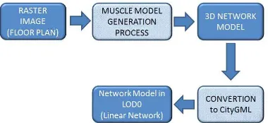
This paper describes the usage of MUSCLE (Multidirectional Scanning for Line Extraction) Model with correction process for automatic generation of 3D networks in CityGML format (from raster floor plans). Once the network generation process completed, the data is converted into CityGML format in LOD0 (Level of Detail). The whole data generation process is described in a flow chart showed in Figure 1. The details of every stages are explained in the following sections.
Figure 1. Data Generation Process
2. MUSCLE MODEL
MUSCLE (Multidirectional Scanning for Line Extraction) Model is a conversion method which was developed to vectorize the straight lines through the raster images including township plans, maps, architectural drawings, and machine plans. Line is one of the most fundamental elements in graphical information systems. In previous studies, there are a large number of algorithms developed for detecting lines from raster images. The vectorization methods implemented in these algorithms can be categorized into following six classes; (1) Hough Transform (HT) based methods, (2) thinning based methods, (3) contour based methods, (4) run-graph based
methods, (5) mesh pattern based methods, and (6) sparse pixel based methods. After the scanning, thresholding, and filtering stages, a traditional vectorization process consists of three stages (except HT based methods); (1) line thinning, (2) line following and chain coding, and (3) vector reduction (i.e. line segment approximation). Unlike traditional vectorization process, this model generates straight lines based on a line thinning algorithm, without performing line following-chain coding and vector reduction stages. In some cases, raster data become unmanageable and the process generates wrongly vectorized lines. In the following sections, the process and correction application explains in detail.
2.1 Threshold Processing
In grayscale images, the objects may contain many different levels of gray tones. In this study, the objects are separated by using the threshold processing technique, with the assumption that the gray values are distributed over the image nearly homogeneous (Wang and Bai, 1999; Belkasim et al, 2003; Liao et al, 2001). In the threshold process, a predetermined gray level (threshold value) is to be determined and every pixel darker than this level is assigned black, while every lighter pixel is assigned white. Therefore, the grayscale image was converted into a binary image (Sun and Wu, 2007, Hasson et al, 2006).
2.2 Horizontal and Vertical Scanning of the Binary Image
In this stage, the horizontal and vertical lines were extracted from the binary image. The nearly vertical lines were obtained by scanning the images horizontally, while the nearly horizontal lines were obtained by scanning the images vertically. The forms of nearly vertical and nearly horizontal
lines are shown in Figure 2. In Figure 2a, the lines which pass through the region 1 and 2 are defined as the nearly vertical lines and the nearly horizontal lines, respectively. Figure 2b and Figure 2c indicates the sample drawings for nearly vertical and nearly horizontal lines, respectively. In other words, if the slope (tangent) of the line is between -1 and +1, it is defined as “nearly horizontal line”. If the slope (tangent) of the line is less than -1 or greater than +1, it is defined as “nearly vertical line”. At the first step, each row on the binary image was scanned horizontally to determine the thickness of the lines and the position of the pixels, which were located in the mid-point of the lines. During this process, the value (black or white) of each pixel was checked by moving from left to right.
Figure 2. Samples of nearly vertical and nearly horizontal lines
Once the first black pixel was met, its column number was stored into the algorithm. While continuing to scan pixels, the column number of the first white pixel was also stored into the algorithm. Thus, the position of the middle pixel in the mid-point of the line could be determined by using the following equation, based on the image coordinate system:
Position of mid pixel = m + Absolute Value ((n - m) / 2) (1)
m: 1st black pixel’s column #, n: 1st white pixel’s column # For example, assuming that 8th pixel is the first black pixel and 13th pixel is the first white pixel in Figure 3a. Using Equation 1, position of the middle pixel can be calculated as 10th pixel, which is then colored with red. After performing the same process for each row on the image, distribution of the red pixels for nearly vertical and nearly horizontal lines are indicated in Figure 3a and Figure 3b, respectively. In these figures, the distribution of the red pixels indicates that the red pixels have continuity for nearly vertical lines; however they have discontinuity for nearly horizontal lines.
Figure 3. Determining red pixels by using horizontal and vertical scanning process.
After the horizontal scanning processes were completed, only the red pixels were selected. Then, a neighborhood analysis was carried out based on the nearly vertical lines by taking the advantages of discontinuity on the nearly horizontal lines. In this method, a red pixel, which is adjacent to another red one, was searched along the lines. This process continued until no red pixels were found adjacent to each other, indicating that the end of the line has been reached. The beginning and ending points of all the nearly vertical lines were determined by using the same procedure.
At the second step, the binary image was scanned vertically, and then, the same process described above was carried out for all columns. Unlike horizontal scanning, the red pixels have continuity for nearly horizontal lines (Figure 3c); however they have discontinuity for nearly vertical lines (Figure 3d). Therefore, the neighborhood analysis was carried out based on the nearly horizontal lines and the beginning and the ending points of all the plenary horizontal lines were determined. After completing the horizontal and vertical scanning of the binary image, the final vectorized data was generated by vectorizing the nearly vertical and the horizontal lines.
3. CORRECTION OF FAULTY LINES
3.1 Detecting Faulty Vectorized Lines
In a case where two or more consecutive lines are nearly horizontal or nearly vertical, raster data becomes unmanageable and the process described in the previous stages generates wrongly vectorized lines. For example, initially, three consecutive nearly horizontal lines (AB, BC, and CD) were horizontally scanned as displayed in Figure 4a. Due to discontinuity of the red pixels between intersection points A, B, C, and D, the neighborhood analysis can not be performed and vectorized data can not be generated. When the raster image was vertically scanned during the second step, the neighborhood analysis yielded wrong vectorization results because of continuity of the red pixels. The algorithm recognizes point A as the beginning point of the line, skips point B and point C, and ends the line at point D. Therefore, the process generates a wrongly vectorized line between point A and D as indicated in Figure 4b.
The detection of wrongly vectorized data is performed by comparing the middle axis of the lines (red pixels) with the vectorized lines. The middle axis and the vectorized line have to be based on the same linear equation. For example, if a sample vectorized line (AB line) is a line with the beginning point of A(Xa,Ya) and the ending point of B(Xb,Yb), then, the linear equation for this vectorized line can be formed as follows:
Figure 4. Detecting wrong vectorization after vertical and horizontal scanning.
(Y- Ya) / (Ya - Yb) = (X- Xa) / (Xa - Xb) (2)
Y = ((Ya - Yb) / (Xa - Xb)) X + ((Yb Xa - Xb Ya) / ( Xa - Xb)) (3)
When X coordinate of a red pixel is inserted into the linear Equation 3, and if the difference between the Y value derived
from this equation and the Y coordinate of this pixel is greater than a user defined maximum deviation, the model defines this line as a wrongly vectorized line. After this process, the red pixels within the acceptable deviation range were eliminated from the image by converting them into the white pixel values. The wrongly vectorized lines with red pixels were remained unchanged within the image.
3.2 Correction of Faulty Vectorized Lines by Using Diagonal Scanning
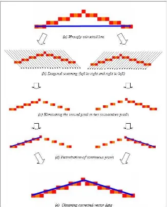
The image having the wrongly vectorized lines (Figure 5a) was diagonally (under 45o angle) scanned; first, from left to right, and then, from right to left (Figure 5b). In diagonal scanning process, if there were two consecutive red pixels along the direction of scanning, the second red pixel is eliminated. Thus, vectorized line took a discontinuous form as shown in Figure 5c. After applying the neighborhood analysis, the lines failed to have the acceptable number of pixels were not vectorized. The continuous pixels, determined by implementing diagonal scanning from both directions, were vectorized as indicated in Figure 5d. Then, corrected vector data was generated by combining both of the vectorized lines together (Figure 5e).
Figure 5. Correction of wrong extracted lines by using diagonal scanning procedure.
4. 3D BUILDING NETWORK CONSTRUCTION 4.1 Generating 3D Network Model
By using the MUSCLE Model described in previous section, the 3D topological Network Model of a building can be constracted automatically from raster floor plans. The user interface of 3D Model Constraction Software is shown in Figure 6.
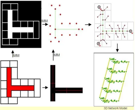
In Network Model, corridor is the main backbone in the floor plan since it connects the rooms with all the other entities in the building. Therefore, determining and modeling the corridor is very important. Once corridor was provided by the user, algorithm leaves only the corridor in the image, and then, determines the middle lines based on the MUSCLE Model. After number of processes on selected middle lines, topological model and coordinates of the corridor are found as seen in Figure 7.
Figure 6. 3D Network Model Construction User Interface
In determining the rooms, corridor is excluded from the image and only the rooms are left. Then, by applying the method, middle point of the rooms are determined and defined as the nodes which represent the rooms Figure 7. After locating the nodes that indicates corridor and rooms, user interactively points out which room nodes connect with which corridor nodes, and geometric network for 2D floor plan is generated. After stairs (or elevator) nodes are indicated by a user, the network is automatically designed by assigning different elevation values for each floor based on various data such as floor number and floor height, and then, 3D NM is generated as seen in Figure 7.
4.2 Converting Network Model into CityGML Format
CityGML is an open data model and XML-based format for the storage and exchange of virtual 3D city models. It is an application schema for the Geography Markup Language version 3.1.1 (GML3), the extendible interna-tional standard for spatial data exchange issued by the Open Geospatial Consortium (OGC) and the ISO TC211 (Gröger et al. 2008).
The aim of the development of CityGML is to reach a common definition of the basic entities, attributes, and relations of a 3D city model. This is especially important with respect to the cost-effective sustainable mainte-nance of 3D city models, allowing the reuse of the same data in different application fields. CityGML not only represents the graphical appearance of city models but specifically addresses the representa-tion of
the semantic and thematic properties, taxonomies and aggregations (Gröger et al. 2008).
Figure 7. 3D Network Generation Process by using MUSCLE Model (MM).
CityGML includes a geometry model and a thematic model. The geometry model allows for the consistent and homogeneous definition of geometrical and topological properties of spatial objects within 3D city models. The base class of all objects is CityObject which is a subclass of the GML class Feature. All objects inherit the properties from CityObject.
CityGML supports different Levels of Detail (LOD). LODs are required to reflect independent data collection processes with differing application requirements (Figure 8). The coarsest level LOD0 is essentially a two and a half dimensional Digital Terrain Model, over which an aerial image or a map may be draped. LOD1 is the well-known blocks model comprising prismatic buildings with flat roofs. In contrast, a building in LOD2 has differentiated roof structures and thematically differentiated surfaces. Vegetation objects may also be represented. LOD3 denotes architectural models with detailed wall and roof structures, balconies, bays and projections. High-resolution textures can be mapped onto these structures. In addition, detailed vegetation and transportation objects are components of a LOD3 model. LOD4 completes a LOD3 model by adding interior structures for 3D objects. For example, buildings are composed of rooms, interior doors, stairs, and furniture (Gröger et al. 2008).
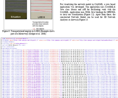
3D Network Model is represented using Transportation Module of CityGML. The transportation model of CityGML is a multi-functional, multi-scale model focusing on thematic and func-tional as well as on geometrical/topological aspects. Transportation features are represented as a linear network in LOD0. Starting from LOD1, all transportation features are geometrically described by 3D surfaces. The main class is transportationComplex, which represents, for example, a road, a track, a railway, or a square. Representation of a TransportationComplex for LOD0 is illustrated in Figure 9 (Gröger et al. 2008).
Figure 8. The five levels of detail (LOD) defined by CityGML (Gröger et al. 2008, source: IGG Uni Bonn).
Figure 9. TransportationComplex in LOD0 (Example shows part of a Motorway) (Gröger et al. 2008)
Once the network generation process completed, the data is converted to and created a CityGML format in LOD0 through program code for writing in a text file by using topological network model details; e.g. nodes, edges and coordinates (Figure 10).
Print #2, "<gml:curveMember><gml:LineString srsDimension=" & Chr(34) & "3" & Chr(34) & "> <gml:posList id=" & Chr(34) & "1" & Chr(34) & ">" &
Fix(xim(fn(th))); Fix(yim(fn(th))); Fix(Val(Text5) + (Val(Text4) * dk)); Fix(xim(tn(th))); Fix(yim(tn(th)));
Fix(Val(Text5) + (Val(Text4) * dk)) &
"</gml:posList></gml:LineString> </gml:curveMember>"
Figure 10. An example line of program code for writing to CityGML file.
3D Network Model is represented as a linear network using Transportation Module of CityGML. Network model in CityGML format is shown in Figure 11.
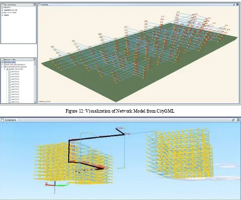
For visualizing the network model in CityGML, a java based application was developed. The application uses CityGML4j Java class library and API for facilitating work with the CityGML. Application uses JOGL Java bindings for OPENGL to carry out visualization (Figure 12). Apart from these, the constracted Network Model can be used for 3D Network Analyses as shown in Figure 13.
Figure 11. Network model represented in LOD-0 linear network in CityGML file.
Figure 12: Visualization of Network Model from CityGML
Figure 13: 3D Network Analyses on the Network Model in CityGML file.
5. CONCLUSIONS
In this study, MUSCLE (Multidirectional Scanning for Line Extraction), was developed by implementing an appropriate computer programming to automatically vectorize the raster data with straight lines. The algorithm of the model generates the line thinning and the simple neighborhood techniques for vectorization processes. When the model works, in some cases raster data become unmanageable and the process generates wrongly vectorized lines. In this situation, to obtain the precise lines, the image with the wrongly vectorized lines is diagonally scanned.
By using this method, the 3D Network models can be constracted topologically in CityGML format from raster floor plans. After the generation process, it is possible to visualize and perform 3D Network Analyses based on these models. In this paper, it was indicated that the MUSCLE Model may successfully be used to generate 3D Topological Network Models of the buildings and convert them into CityGML data format.
6. REFERENCES
Belkasim, S.; Ghazal, A.; Basir, O.A. Phase-based optimal image thresholding. Digit. Signal Process. 2003, 13, 636–655. Gröger, G., Kolbe, T.H., Czerwinski, A., Nagel, C., 2008. OpenGIS City Geography Markup Language (CityGML) Encoding Standard, Version 1.0.0, International OGC Standard. Open Geospatial Consortium.
Hasson, N.N.; Aljunid, S.A.; Badlishah, A. R., 2006, Simplification of Raster Images to Extract Visual Information. International Journal of Computer Science and Network Security , 6(11), p.49.
Liao, P.S.; Chen, T.S., 2001, Chung, P.C. A Fast Algorithm for Multilevel Thresholding. J. Inf. Sci. Eng. , 17, 713-727. Sun, J. and Wu, X., 2007, Shape Retrieval Based on the Relativity of Chain. Lect. Notes Comput. Sc. 2007, V. 4577, P. 76-84
Wang, L.; Bai, J. Threshold selection by clustering gray levels of boundary. Pattern Recogn. Lett. 2003, 24(12), 1983–1999