Two-Field Integrable Evolutionary Systems of
the Third Order and Their Dif ferential Substitutions
Anatoly G. MESHKOV and Maxim Ju. BALAKHNEV
Orel State Technical University, Orel, Russia
E-mail: a [email protected], [email protected]
Received October 04, 2007, in final form January 17, 2008; Published online February 09, 2008 Original article is available athttp://www.emis.de/journals/SIGMA/2008/018/
Abstract. A list of forty third-order exactly integrable two-field evolutionary systems is presented. Differential substitutions connecting various systems from the list are found. It is proved that all the systems can be obtained from only two of them. Examples of zero curvature representations with 4×4 matrices are presented.
Key words: integrability; symmetry; conservation law; differential substitutions; zero cur-vature representation
2000 Mathematics Subject Classification: 37K10; 35Q53; 37K20
1
Introduction
We use the term “integrability” in the meaning that a system or equation under consideration possesses a Lax representation or a zero curvature representation. Such systems can be solved by the inverse spectral transform method (IST) [1,2]. Exactly integrable evolution systems are of interest both for mathematics and applications. In particular, systems of the following form
ut=uxxx+F(u, v, ux, vx, uxx, vxx), vt=a vxxx+G(u, v, ux, vx, uxx, vxx), (1.1)
whereais a constant, excite great interest since about 1980. The paper [3] is devoted to construc-tion of systems of the form (1.1) among others. Nine integrable systems of the form (1.1) and their Lax representations have been obtained in the paper. In particular, it contains a complete list of three integrable systems (1.1) satisfying the conditions a(a−1)6= 0 and ord(F, G) <2. Here ord = order, ordf < nmeans thatf does not depend onun, vn, un+1, vn+1, . . .. Here and in what follows, the notations un=∂nu/∂xn,vn=∂nv/∂xn are used.
Two of the three mentioned systems can be written in the following form
ut=u3+v u1, vt=−12v3+u u1−v v1, (1.2)
ut=u3+v u1, vt=−12v3−v v1+u1 (1.3)
and the third system is presented below (see (3.46a)). System (1.2) was found independently in [4] and the soliton solutions were constructed there. This system is called as the Drinfeld– Sokolov–Hirota–Satsuma system.
This paper contains two results: (i) a list of integrable systems of the form (1.1) with smooth functions F,Gand a=−1/2; (ii) differential substitutions that allow to connect any equation from the list with (1.2) or (1.3).
number of constants some of which can be removed by scaling and linear transformations. Note that there are two-field integrable evolutionary systems ut=Au3+H(u,u1,u2) with a
non-diagonal main matrix A. For example, an integrable evolutionary system with the Jordan main matrix is found in [14].
Moreover, about 50 two-field integrable systems of the form (1.1) witha= 1 can be extracted from papers [15,16,17,18,19] that deal with vector evolutionary equations.
Partial solutions of the classification problem for a= 0 and ordG 61 have been obtained in [20], and in [21] for divergent systems witha6= 1. A complete list of integrable systems of the form (1.1) does not exist today because the problem is too cumbersome and the set of integrable systems is very large.
Our tool is the symmetry method presented in many papers. We shall point out pioneer or review papers only. In [22] the notions of formal symmetry and canonical conserved density for a scalar evolution equation are introduced. These tools were applied to classification of the KdV-type equations in [23]. A complete theory of formal symmetries and formal conservation laws for scalar equations has been presented in [24]. A generalized theory was developed for evolutionary systems in [25]. Review paper [26] contains both general theorems of the symmetry method and classification results on integrable equations: the third and fifth order scalar equations, Schr¨odinger-type systems, Burgers-type equations and systems. Review paper [27] is devoted to higher symmetries, exact integrability and related problems. Peculiarities of systems (1.1) have been discussed in [21]. For the sake of completeness, the main points of the symmetry method and some results necessary for understanding of this paper are considered in the Sections 2–4.
Briefly speaking, the symmetry method deals with the so-called canonical conservation laws
Dtρn=Dxθn, Dtρ˜n=Dxθ˜n, n= 0,1,2, . . . , (1.4)
where Dt is the evolutionary derivative and Dx is the total derivative with respect to x. In particular, ρ0 =−Fu2/3, ˜ρ0 =−Gv2/(3a). The recursion relations for the canonical conserved
densities ρn and ˜ρn are presented in Section2. All canonical conserved densities are expressed in terms of functions F and G. That is why equations (1.4) impose great restrictions on the forms of F and G. Equations (1.4) are solvable in the jet space iff
EαDtρn= 0, EαDtρ˜n= 0, α= 1,2, n= 0,1,2, . . . (1.5)
(see [28], for example). Here
Eα ≡
δ δuα =
∞ X
n=0
(−Dx)n
∂ ∂uα
n
, (u1 =u, u2 =v),
is the Euler operator.
Conservation law with ρ = Dxχ, θ =Dtχ is called trivial and the conserved density of the formρ=Dxχis called trivial too. This can be written in the formρ∈ImDx, where Im = Image. If ρ1−ρ2∈ImDx, then the densitiesρ1 and ρ2 are said to be equivalent.
There are a lot of systems in the following form
ut=uxxx+F(u, ux, uxx), vt=a vxxx+G(u, v, ux, vx, uxx, vxx),
The system of two independent equations
ut=uxxx+F(u, ux, uxx), vt=a vxxx+G(v, vx, vxx),
will be called disintegrated. It is obvious that the disintegrated form is a partial case of the triangular form. Therefore the disintegrated systems and those reducible to them have been omitted.
System (1.1) will be called reducible if it is triangular or can be reduced to triangular or disintegrated form. Otherwise, the system will be called irreducible.
Our computations show that for irreducible integrable systems (1.1) parameteramust belong to the following set:
A=n0, −2, −12, −72+ 32√5, −72 −32√5o.
These values were found first in [3] and were repeated in [29]. The value ofais always defined at the end of computations when functionsF andGhave been found and only some coefficients are to be specified from the fifth or seventh integrability conditions (see example in Section3.1). This means that it is enough to verify conditions (1.5) forn= 0, . . . ,7 andα = 1,2 to obtainF,G
and a. But for absolute certainty we have verified conditions (1.5) for n= 8,9 andα = 1,2 for each system.
The presented set A consists of zero and two pairs (a, a−1). The transformation t′ = at,
u′ = v, v′ = u changes the parameter a 6= 0 in (1.1) into a−1. That is why one ought to consider the values
0, −12, −72 +32√5 of the parameter a. Integrable systems with a = 0 were mentioned above, see also [30]. This paper is devoted to investigation of the casea=−1/2 only. The casea=−72 +32√5 will be presented in another paper.
Section 2 contains recursion formulas for the canonical densities. The origin of the notion, some examples and a preliminary classification are considered.
A list of forty integrable systems and an example of computations are presented in Section3. Section 4 contains differential substitutions that connect all systems from the list. The method of computations and an example are considered. It is shown that all systems from the list presented in Section3 can be obtained from (1.2) and (1.3) by differential substitutions.
Section 5 is devoted to zero curvature representations. The zero curvature representations for systems (1.2) and (1.3) are obtained from the Drinfeld–Sokolov L-operators. A method of obtaining zero curvature representations for other systems is demonstrated.
2
Canonical densities
One of the main objects of the symmetry approach to classification of integrable equations is the infinite set of the canonical conserved densities. Let us demonstrate how canonical conserved densities can be obtained the from the asymptotic expansions for eigenfunctions of the Lax operators. The simplest Lax equations concerned with the KdV equation
ut= 6uux−uxxx
take the following form
ψxx−uψ−µ2ψ= 0, (2.1)
ψt=−4ψxxx+ 6uψx+ 3uxψ+ 4µ3ψ. (2.2)
Here u is a solution of the KdV equation andµis a parameter. The standard substitution
ψ= exp Z
ρ dx
reduces equations (2.1) and (2.2) to the Riccati form
ρx+ρ2−u−µ2 = 0, (2.3)
∂t Z
ρ dx=−4(∂x+ρ)2ρ+ 6uρ+ 3ux+ 4µ3. (2.4)
Differentiating temporal equation (2.4) with respect tox one can rewrite it, using (2.3), as the continuity equation:
ρt=∂x[(2u−4µ2)ρ−ux]. (2.5)
To construct an asymptotic expansion one ought to set
ρ=µ+ ∞ X
n=0
ρn(−2µ)−n. (2.6)
Then equation (2.3) results in the following well known recursion formula [2]
ρn+1 =Dxρn+ n−1 X
i=1
ρiρn−i, n= 1,2, . . . , ρ0= 0, ρ1 =−u, (2.7)
and (2.5) results in infinite sequence of conservation laws:
Dtρn=Dx(2uρn−ρn+2), n >0. (2.8)
We change here ∂t → Dt and ∂x → Dx because u is a solution of the KdV equation. The obtained conservation laws are canonical. It is easy to obtain several first canonical densities:
ρ2=−u1, ρ3 =u2−u2, ρ4=Dx(2u2−u2), . . . .
It is shown in [2] that all even canonical densities are trivial. Note that if one chooses an-other asymptotic expansion, for example, in powers ofµ−1 instead of (2.6), then another set of canonical densities is obtained, which is equivalent to the previous set.
The canonical densities that follow from (2.7) can also be obtained by using the temporal equation (2.4) only. Indeed, setting ∂tR ρ dx=θone obtains from (2.4)
−4(∂x+ρ)2ρ+ 6uρ+ 3ux+ 4µ3 =θ. (2.9)
Using the same expansions as above
ρ=µ+ ∞ X
n=0
ρn(−2µ)−n, θ= ∞ X
n=0
θn(−2µ)−n,
one can obtain from (2.9) the following recursion relation:
ρn+2 = 2uρn+ 2 n+1 X
i=0
ρiρn−i+1−43 n X
i,j=0
ρiρjρn−i−j− 13θn
+ 2Dx ρn+1− n X
i=0
ρiρn−i !
−4 3D
2
xρn−uδn,−1+u1δn0, n=−2,−1,0, . . . ,
n >2 depend on θn−2. The fluxes θn must be defined now from equations (1.4). For example,
θ1 =u2−3u2.
The traditional method to obtain the canonical densities for an evolution system [25]
ut=K(u,ux, . . . , un), u(t, x)∈Rm, m>1, uα
k =∂xkuα. (2.10)
consists, briefly, in the following. The main idea is to use the linearized equation
(Dt−K∗)ψ= 0 (2.11)
or its adjoint
(Dt+K+∗)ϕ= 0 (2.12)
as the temporal Lax equation. Here
(K
∗ψ)α = X
n,β
∂Kα ∂uβn
Dxnψβ, (K+
∗ϕ)α= X
n,β
(−Dx)n∂K β
∂uα n
ϕβ,
Dt=
∂ ∂t +
X
n,α
Dnx(Kα) ∂
∂uα n
, Dx =
∂ ∂x+
X
n,α
uαn+1 ∂ ∂uα
n
.
The spatial Lax operator (formal symmetry) was introduced in [25] as the infinite operator series
R= N X
k=−∞
RkDxk, N >0, (2.13)
commuting with Dt−K∗. Rk are matrix coefficients depending on u,ux, . . .. It was shown that Tr resR (resR=R−1) is the conserved density for system (2.10). Canonical densities have been defined by the formulas
ρn= Tr resRn, n= 1,2, . . . ,
see [26] for details.
Operations with operator series (2.13) are not so simple, therefore we use an alternative method for obtaining the canonical densities. It was proposed in [32] heuristically and we present the following explanation (see also [33]).
Observation. One can obtain equation (2.9) from (2.2) by the following substitution
ψ=eω, ω= Z
ρ dx+θ dt, (2.14)
whereρ dx+θ dtis the smooth closed 1-form, that is,Dtρ=Dxθ. This impliese−ωDteω =Dt+θ,
e−ωD
xeω =Dx+ρand so (2.9) follows. Another way to obtain the same equation is to prolong the operators Dt → ∂t+θ,Dx → ∂x+ρ in (2.2) formally and to set ψ = 1. For systems, one must setψα= 1 for a fixed α only.
We shall apply this method to system (1.1) now.
The linearized system (1.1) with prolonged operators Dx →Dx+ρ,Dt→ Dt+θ takes the following form:
(Dx+ρ)3+Fu+Fu1(Dx+ρ) +Fu2(Dx+ρ) 2−D
t−θΨ1 +
Fv+Fv1(Dx+ρ) +Fv2(Dx+ρ) 2
If one sets here Ψ1= 1, then the first equation takes the following form
(Dx+ρ)2ρ+Fu+Fu1ρ+Fu2(Dx+ρ)ρ−θ
+
Fv+Fv1(Dx+ρ) +Fv2(Dx+ρ) 2
Ψ2 = 0.
It is obvious from this equation that the following forms of the asymptotic expansions are acceptable:
Here µ is a complex parameter. Then, after some simple calculations, the following recursion relations are obtained (n>−1):
+ 3a Dx n X
i=0
ρiϕn−i+a n X
i=0
ϕn−iDx2ρi+a n X
i+j+k=0
ρiρjρkϕn−i−j−k.
Here δi,k is the Kronecker delta, Fu1 = ∂F/∂u1 and so on. From the recursion relations it is
obvious why the valuea= 1 is singular. Some of initial elements of the sequence{ρn, ϕn} read
ρ0=−13Fu2, ϕ0 = 0, ϕ1 =
1
1−aGu2,
others are introduced via the δ-symbols.
If one sets in (2.15) Ψ2 = 1 anda6= 0, then one more pair of recursion relations for{ρ˜n,ϕ˜n} is obtained. These recursion relations give us any desired number of canonical densities. As an example, we present here some more canonical densities:
ρ0=− 1
3Fu2, ρ1 =
1 9F
2 u2 −
1 3Fu1+
1
3bFv2Gu2+
1
3DxFu2,
˜
ρ0=− 1
3aGv2, ρ˜1=
1 9a2 G
2 v2−
1
3aGv1 −
1
3a bFv2Gu2 +
1
3aDxGv2, (2.16)
where b=a−1. The tilde denotes another sequence of canonical densities. Further canonical densities are too cumbersome, therefore we do not present them here.
To simplify investigation of the integrability conditions, an additional requirement is always imposed. This is the existence of a formal conservation law [25,26]. A formal conservation law is an operator series N in powers of D−1
x . An equation for the formal conservation law can be written in the following operator form
(Dt−K∗)N =N(Dt+K∗+). (2.17)
The form of this equation coincides with the form of the equation for the Noether operator [34]. That is a formal conservation law may be called a formal Noether operator.
If (Dt−K∗, L) is the Lax pair for an equation, then (Dt+K∗+, L+) is obviously the Lax pair for the same equation. Hence, canonical densities obtained from (2.11) must be equivalent to canonical densities obtained from (2.12).
It was shown in [21] that the first sequence of the canonical densities ρn for system (1.1) obtained from (2.11) is equivalent to the first sequence of the canonical densities τn obtained from (2.12) and the second sequence of the canonical densities ˜ρn is equivalent to the second sequence of the canonical densities ˜τn. Hence,ρn−τn∈ImDx and ˜ρn−τ˜n∈ImDx, or
Eα(ρn−τn) = 0, Eα(˜ρn−τ˜n) = 0, α= 1,2, n= 0,1,2, . . . . (2.18)
Equations (1.4) (or (1.5)) and (2.18) are said to be the necessary conditions of integrability. We shall refer to it simply as the integrability conditions for brevity.
Our computations have shown that
τ0 =−ρ0, ˜τ0=−ρ˜0, τ1 =ρ1, ˜τ1= ˜ρ1. (2.19)
Other “adjoint” canonical densities τi and ˜τk essentially differ from the “main” canonical den-sities ρi and ˜ρk. All canonical densities can be obtained using the Maple routines cd and acd from the package JET (see [36]). These routines generate the “main” and the “adjoint” canon-ical densities, correspondingly, for almost any evolutionary system (an exclusion is the case of multiple roots of the main matrix of the system under consideration).
Thus, according to (2.16) and (2.19) we have Fu2 ∈ImDx and Gv2 ∈ ImDx (a6= 0). This
Lemma 1. System (1.1) with a(a−1)6= 0 satisfying the zeroth integrability conditions (2.18)
reads
ut=u3− 3
2f u2Dxf+
3 4f fu1u
2
2+F1(u, v, u1, v1, v2),
vt=av3− 3a
2gv2Dxg+
3a
4ggv1v 2
2 +G1(u, v, u1, v1, u2). (2.20)
where ord(f, g)61.
Indeed, one may setFu2 =−3/2Dxlnf andGv2 =−3/2aDxlng, where ord(f, g)61 because
ord(F, G)62. Then equations (2.20) follow.
From higher integrability conditions one more lemma follows.
Lemma 2. Suppose system (2.20) is irreducible and satisfies the following eight integrability conditionsρ2−τ2 ∈ImDx,ρ˜2−τ˜2 ∈ImDx andDtρn∈ImDx,Dtρ˜n∈ImDx, wheren= 1,3,5.
Then the system must have the following form
ut=u3− 3
2f u2Dxf+
3 4f fu1u
2
2+f1v22+f2v2+f3,
vt=av3− 3a
2gv2Dxg+
3a
4ggv1v 2
2 +g1u22+g2u2+g3, a6= 0, (2.21)
where ord(f, g, fi, gj)61.
A scheme of the proof has been presented in [21].
3
List of integrable systems
As it is shown in Section 2 the problem of the classification of integrable systems (1.1) is reduced to investigation of system (2.21). That is why it is necessary to start by investigating its symmetry properties.
Lemma 3. System (2.21) are invariant under any point transformation of the form
(a) t′ =α3t+β, x′ =αx+γt+δ, α6= 0, u′ =u, v′ =v, (b) u′ =h
1(u), v′ =h2(v),
and under the following permutation transformation
(c) t′=at, u′ =v, v′ =u,
where α, β, γ and δ are constants,hi are arbitrary smooth functions.
The classification of systems of type (2.21) has been performed by modulo of the presented transformations.
Moreover, some systems (2.21) admit invertible contact transformations. An effective tool for searching such contact transformations is investigation of the canonical conserved densities. For example, system (3.24) from the next section has the first canonical conserved density of the following form:
ρ1= v1−23uev2+ 2c21e−2v.
It is obvious that the best variables for that system are
This is an invertible contact transformation. In terms ofU andV the system takes the following simple form:
Ut=Dx U2+32U V1−34U V2+12c21U3
,
Vt= 14Dx(V3−2V2)−32c21Dx(2U U1+U2V).
Ifc1 6= 0 this system can be reduced to (3.10) by scaling, otherwise the system is triangular: the equation for V will be independent single mKdV. Moreover, the equation forU becomes linear. That is why c1 6= 0 in (3.24).
Canonical densities for the triangular systems contain only one highest order term in the second power as in the considered exampleρ=V2 orρ=Vx2+· · ·, orρ=Vxx2 +· · · etc. Trian-gular systems and those reducible to the trianTrian-gular form have been omitted in the classification process as trivial.
To classify integrable systems (1.1) with a(a−1) 6= 0 one must solve a huge number of large overdetermined partial differential systems for eight unknown functions of four variables. This work has required powerful computers and has taken about six years. All the calculations have been performed in the interactive mode of operation because automatic solving of large systems of partial differential equations is still impossible. The package pdsolve from the excellent system Maple makes errors solving some single partial differential equations. The packagediffalgcannot operate with large systems because its algorithms are too cumbersome. Thus, one has to solve complicated problems in the interactive mode. Hence, to obtain a true solution one must enter true data! Under such circumstances errors are probable. The longer the computations the more probable are errors. This is the reason why we cannot state with confidence that all computations have been precise all these six years. That is why the statement on completeness of the obtained set of integrable systems is formulated as a hypothesis.
In this and in the following sectionsc,ci,k,ki are arbitrary constants.
Hypothesis. Suppose system (2.21) with a=−1/2 is irreducible. If the system has infinitely many canonical conservation laws, then it can be reduced by an appropriate point transformation to one of the following systems:
ut=u3+v u1, vt=−12v3+u u1−v v1; (3.1)
ut=u3+v1u1, vt=−12v3+12(u2−v21); (3.2)
ut=u3+v u1, vt=−12v3−v v1+u1; (3.3)
ut=u3+v u1+v1u, vt=−12v3−v v1+u; (3.4)
ut=u3+v1u1, vt=−12v3−12v12+u; (3.5)
ut=u3+u u1+v1, vt=−12v3+32u1u2−u v1; (3.6)
ut=u3+v2+k u1, vt=−12v3+32uu2+34u21+13u3+k u2−v1
; (3.7)
ut=u3+32vv2+34v21+13v
3−k v2+u
1, vt=−12v3+u2+k v1; (3.8)
ut=u3−32u1v2−43u1v12+14u31, vt=−12v3+ 32u1u2−43u21v1+14v13; (3.9)
ut= u2−32uv1− 34uv2+14u3
x, vt= − 1
2v2+32uu1−34u 2v+1
4v 3
x; (3.10)
ut=u3−32v2− 32u1v1−12u31, vt=−12v3+32 v1−u2+12u21 2
−34v21; (3.11)
ut= u2−32v1−23uv−12u3x, vt=
−12v2+32 v−u1+12u2 2
−34v2
x; (3.12)
ut=u3−3gv2−3u1(u1+v1)−32v12−6v1g2−c1g3−3g4,
vt=−12v3−34c1u2+ 3u21−32v 2
1−6u1g2+c1g3+ 3g4, g=u+v; (3.13)
ut=u3−3u1v1+ (u−3v2)u1, vt=−12v3+12u2−u1v−(u−3v2)v1; (3.14)
ut=u3−32u1v2−34u1v12+14u 3
1−c1e−2vu1−c2(u1+ 2v1)e2(u+v) +c3(u1−2v1)e2(v−u),
vt=−12v3+32u1u2− 34u21v1+14v13+c1e−2vv1+ c2e2(u+v)−c3e2(v−u)v1; (3.31)
ut=u3−32u1v2−34u1v12+41u31+ c2eu+c3e−u−3c21e−2v
u1,
vt=−12v3+23u1u2− 34u21v1+14v13+ c2eu−c3e−uu1 + 3c21e−2v−c
2eu−c3e−u
v1; (3.32)
ut=u3−32u1v2−34u1v12+14u 3
1+ 3k(u21−2v2)e−v−3(c2−3k2)u1e−2v + 8k(k2−c2)e−3v,
vt=−12v3+32u1u2− 34u21v1+14v13+ 3k(u2−2u1v1)e−v+ 3(c2−3k2)v1e−2v; (3.33)
ut=u3−32u1v2−34u1v12+14u31−3c21u1e2(u+v)+ 3c1u1(u1+ 2v1)eu+v + (c2e−u−3c32e−2v)u1,
vt=−12v3+32u1u2− 34u21v1+14v13+ 3c21(2u1+v1)e2(u+v)+ 3c1(u2+u21)eu+v
−c2(u1+v1)e−u+ 3c23v1e−2v; (3.34)
ut=u3−32u1v2−34u1v12+14u31+ 3c2u1(u1+ 2v1)eu+v−4c1c2e3(u+v) + 3[(c1−c22)u1+ 2c1v1]e2(u+v),
vt=−12v3+32u1u2− 34u21v1+14v13+ 3c2(u2+u21)eu+v+ 4c1c2e3(u+v)
+ 3[2c22u1−(c1−c22)v1]e2(u+v); (3.35)
ut=u3−32u1v2−34u1v12+14u13+23c21u1e−2v+c1(2v2−u21)e−v −2c1c2(u1+ 2v1)eu+ 3c2u1(u1+ 2v1)eu+v−3c22u1e2(u+v),
vt=−12v3+32u1u2− 34u21v1+14v13− 23c21v1e−2v+c1(2u1v1−u2)e−v
−2c1c2(u1−v1)eu+ 3c2(u2+u12)eu+v+ 3c22(2u1+v1)e2(u+v); (3.36)
ut=u3−32u1v2−34u1v21+14u31−3u1
c21e2(u+v)+c22e2(v−u)+ 2c1c2e2v
−3c23u1e−2v+ 3c1u1(u1+ 2v1)eu+v−3c2u1(u1−2v1)ev−u,
vt=−12v3+32u1u2− 34u21v1+14v13+ 3c21(2u1+v1)e2(u+v)+ 6c1c2v1e2v
+ 3c22(v1−2u1)e2(v−u)+ 3c1(u2+u21)eu+v+ 3c2(u21−u2)ev−u+ 3c23v1e−2v; (3.37)
ut=u3−32u1v2−43u1v12+14u31−6c31e3(u+v)−34c21(5u1−8v1)e2(u+v)
+92c1u1(u1+ 2v1)eu+v+ 2c21c2e2u+v+23c1c22eu−v−21c1c2(7u1+ 12v1)eu +c2(2v2−u21)e−v+1112c22u1e−2v−92c32e−3v,
vt=−12v3+23u1u2− 34u21v1+14v13+ 6c13e3(u+v)+34c 2
1(18u1+ 5v1)e2(u+v) + 92c1(u2+u21)eu+v−4c21c2e2u+v+23c1c22eu−v−27c1c2(u1−v1)eu
+c2(2u1v1−u2)e−v−1112c22v1e−2v; (3.38)
ut=u3−32u1v2−34u1v12+14u13+c3e−v(u21−2v2) +23c23u1e−2v +c1 3u1eu+v+ 2c3eu
(u1+ 2v1)−c2(3u1ev−u+ 2c3e−u)(u1−2v1) −3u1(c1eu+c2e−u)2e2v,
vt=−12v3+32u1u2− 34u21v1+14v13+c3e−v(u2−2u1v1)− 23c23v1e−2v + 3c21e2(u+v)(2u1+v1)−3c22e2(v−u)(2u1−v1) + 3c1eu+v(u2+u21)
ut=u3−34
(2g3−u2+ 2gv1)2
u1−g2
+ 3g(u2−v2)−6u12−9u1v1−32v12
−3(5g2+ 4cg+c2)u1−6g2v1+ 2cg2(8g+ 3c) + 9g4,
vt=−12v3+34
(2g3−u2+ 2gv1)2
u1−g2 −
3(3g+c)u2−32v12+ 3(9g2+ 8cg+ 2c2)u1
+ 3(6g2+ 4cg+c2)v1−2cg2(8g+ 3c)−9g4, g=u+v; (3.40)
Remark 1. Systems (3.1), (3.3), (3.6) and (3.20) were proposed in [3], where system (3.20) is given with a misprint. System (3.10) was presented in [29].
Remark 2. Ten pairs of integrability conditions (for ρ0–ρ9 and ˜ρ0–˜ρ9) have been verified for each system (3.1)–(3.40), and nontrivial higher conserved densities with orders 2, 3, 4 and 5 have been found.
Remark 3. It is shown in [21] that systems (3.10) and (3.12) are unique divergent systems of the form (2.21) that satisfy the integrability conditions.
Remark 4. System (3.22) is a modification of (3.11), systems (3.31)–(3.39) are modifications of (3.9).
Remark 5. Canonical densities for system (3.25) depend on the nonlocal variablew=D−1 x e−v.
Remark 6. Many of the systems possess discrete symmetries. They are:
u→ −u for (3.1), (3.2), (3.9), (3.10), (3.16), (3.20) and (3.27);
u→ −u,v →v+πifor (3.24);
u→iu,v→v− 2iπ,c1→ −c1 for (3.28);
{u→ −u, v →v+πi} ∪ {v→v+πi, c1 → −c1} ∪ {u→ −u, c1 → −c1}for (3.29); {u→ −u, v →v+πi} ∪ {u→iu, v→v−2iπ} for (3.30);
u→ −u,c2→c3,c3 →c1 for (3.32);
u→ −u,k→ −kfor (3.33);
u→ −u,c1→c2,c2 →c1 for (3.37);
u→ −u,c3→ −c3,c2 →c1,c1 →c2 for (3.39).
Also, systems (3.1), (3.2), (3.9), (3.10) and (3.27) preserve the real shape under the transfor-mation u→iu. System (3.33) keeps the real shape under the transformationu→iu,k→ik.
3.1 Example of computations
Let us consider the simplest case of system (1.1):
ut=u3+f1(u, v)u1+f2(u, v)v1, vt=av3+g1(u, v)u1+g2(u, v)v1, (3.41)
where a(a−1)6= 0. Formulas (2.16) are reduced now to the following
ρ0= 0, ρ˜0 = 0, ρ1=− 1
3f1, ρ˜1 =− 1
3ag2. (3.42)
The further canonical densities read
ρ2=− 1
3(f1,uu1+f2,uv1) + 1
3Dxf1, ρ˜2 =− 1
3a(g1,vu1+g2,vv1) +
1 3aDxg2, τ2 =
1
3(f1,uu1+f2,uv1), τ˜2 = 1
3a(g1,vu1+g2,vv1), (3.43)
The first integrability condition (1.5) for ρ1 can be split with respect to u3, v3, u2 and v2. This provides the following equations
f1,uv= 0, f1,uuu= 0, f1,vvv = 0, or f1(u, v) =c1u2+c2u+c3v2+c4v+c5.
Analogously, condition (1.5) for ˜ρ1 impliesg2(u, v) =b1u2+b2u+b3v2+b4v+b5. It is obvious from (3.43) that the second integrability conditions (2.18) areτ2∈ImDxand ˜τ2 ∈ImDx. These conditions provide f2,uu =g1,vv = 0 orf2(u, v) =uf3(v) +f4(v),g1(u, v) =vg3(u) +g4(u).
Thus, system (3.41) takes the following form:
ut=u3+ (c1u2+c2u+c3v2+c4v+c5)u1+ (uf3(v) +f4(v))v1,
vt=av3+ (vg3(u) +g4(u))u1+ (b1u2+b2u+b3v2+b4v+b5)v1. (3.44)
Now one can obtain θ2 = Dx−1Dtρ2 and ˜θ2 = D−x1Dtρ˜2 in an explicit form. The expres-sionsDtρ1 and Dtρ˜1 are not the total derivatives yet:
Dtρ1=Dxh1(ui, vj) +R1(u, v, u1, v1) =Dxθ1,
Dtρ˜1=Dx˜h1(ui, vj) + ˜R1(u, v, u1, v1) =Dxθ˜1.
Therefore, we have set θ1 =h1(ui, vj) +q1(u, v), ˜θ1 = ˜h1(ui, vj) + ˜q1(u, v), whereq1 and ˜q1 are unknown functions and Dxq1 =R1, Dxq˜1 = ˜R1. This trick allows us to evaluate ρ4, τ4, ˜ρ4, ˜τ4 and verify the fourth integrability conditions (2.18). These conditions implyf′′
3 =g′′3 = 0, hence
f3 =a1v+a2, g3 =a3u+a4.
To simplify the further analysis one must list all irreducible cases of f1 (or g2). Let us take
f1 =c1u2+c2u+c3v2+c4v+c5 for definiteness.
Lemma 4. Using complex dilatations of u andv, translations u→u+λ1, v→v+λ2 and the
Galilei transformation ut→ut+αux, vt →vt+αvx one can reduce f1 to one of the following
forms:
1) u2+v2; 2)u2+αv; 3)v2+αu; 4) u+v; 5)u; 6)v; 7) f1 = 0,
where αis any constant. Moreover, in the cases 4–7the function g2 must be linear(b1 =b3 = 0)
because otherwise the permutation u↔v gives one of the cases 1–3.
In cases 1 and 3 contradictions follow from the integrability conditions (1.5) with n = 1,3 and (2.18) withn= 2,4. In case 2 the integrability conditions (1.5) withn= 1,3,5 and (2.18) withn= 2,4 are satisfied iff system (3.44) is reduced to a pair of independent equations. Thus, a nontrivial integrable system (3.41) must belong to the following class:
ut=u3+ (c2u+c4v)u1+ (u(a1v+a2) +f4(v))v1,
vt=av3+ (v(a3u+a4) +g4(u))u1+ (b2u+b4v+b5)v1, (3.45)
and only the following cases are possible:
4)c2 =c4 = 1; 5)c2 = 1, c4 = 0; 6)c2= 0, c4= 1; 7)c2=c4= 0.
In case 4 the integrability conditions (1.5) withn= 1, . . . ,5 provide the functionsg4=k1u+k2,
f4 =k3v+k4, the coefficients a3 = 0,a4 =−1 +a2+b2,b4 =b2= (a+ 1)a2−2a−1 and the following equations:
a5(a2−2)−a4(4a22−7a2−6)−2a3(16a22−5a2−37)
−a2(177a22−224a2−41)−a(236a22−353a2+ 102)−a2(37a2−53)−17 = 0.
Using the package Groebner in Maple, one can obtain a2 = (1−a)/3, a2 + 7a+ 1 = 0 or
a= (3c−7)/2,c2 = 5. Then, the remaining coefficients are also determined and we obtain
ut=u3+ (u+v)u1+12 (3−c)u+ (5c−11)vv1, c2= 5,
vt= 12v3(3c−7) + (c+ 2)u−v
u1+ 12(c−3)(u+v)v1. (3.46)
The following substitution
V = 16(c+ 1)(v−u), U = 121 (c+ 3)u+16v
reduces system (3.46) to the third Drinfeld–Sokolov system
Ut=−8U3+ 3V3+ 6(V −8U)U1+ 12U V1,
Vt= 12U3−2V3+ 48V U1+ 12(2U −V)V1 (3.46a)
that has been presented first in [3]. Scaling
t→ −12t, U =→ 16U, V =→ −13V
gives more symmetric form of system (3.46a)
Ut= 4U3+ 3V3+ (4U +V)U1+ 2U V1,
Vt= 3U3+V3−4V U1−2(V +U)V1 (3.46b)
that was found in [14].
In case 5 the equations a1 = a2 = 0, g4′f4′ = 0, g′′′4 = 0 follow from the integrability condi-tions (1.5) withn= 1, . . . ,5. This implies f46= 0 because otherwise the first equation of (3.45) will be independent. Hence, there are two branches (1) f4 = 1 and (2) f4′ 6= 0, g4′ = 0. Along the first branch, if one use additionally the integrability conditions (1.5) withn= 7 and solves a large polynomial system for constants, one can obtain the following system:
ut=u3+uu1+v1, vt=−2v3−uv1,
that can be transformed to (1.3) by a scaling.
Along the second branch the integrability conditions (1.5) with n = 1, . . . ,5 provide the following system
ut=u3+uu1−vv1, vt=−2v3−uv1,
that is equivalent to (1.2).
Case 6 is symmetric to case 5: one can obtainf′′′
4 = 0, g4′′ = 0, a3 =a4 =b2 = 0 from the integrability conditions (1.5) withn= 1, . . . ,5. Henceg4 6= 0 and we have two branches g4 = 1 or g4 = u. Using the additional integrability conditions (1.5) with n = 6,7 one can obtain equations (1.2) and (1.3).
4
Dif ferential substitutions
A differential substitution is a pair of equations
u=f(U, V, Ux, Vx, . . . , Un, Vn), v=g(U, V, Ux, Vx, . . . , Un, Vn), (4.1)
where f and gare some smooth functions.
Definition 1. If for any solution (U, V) of a system (Σ) formulas (4.1) provide a solution (u, v) of system (1.1), then one says that system (1.1) admits substitution (4.1).
In all cases that we know, the new systems (Σ) belong to the same class (1.1)
Ut=Uxxx+P(U, V, Ux, Vx, Uxx, Vxx), Vt=a Vxxx+Q(U, V, Ux, Vx, Uxx, Vxx), (S)
with some smooth functions P and Q. There exist some group-theoretical explanation of this fact for KdV type equations [35]. Our attempts to introduce another parameter a′ 6= ain (S) had no success.
Substituting (4.1) into (1.1) one obtains the following equations
Dx3f +F(f, g, Dxf, Dxg, Dx2f, D2xg)−∂tf S
= 0,
aD3xg+G(f, g, Dxf, Dxg, Dx2f, D2xg)−∂tg
S
= 0. (4.2)
It is obvious that transition to the manifold (S) in (4.2) is equivalent to a replacement of∂tby the evolutionary differentiation Dt performed in accordance with (S):
Dtf =Dx3f+F(f, g, Dxf, Dxg, Dx2f, D2xg),
Dtg=aDx3g+G(f, g, Dxf, Dxg, D2xf, D2xg), (4.3)
where
Dtf = n X
i=1
∂f ∂Ui
Dix(U3+P) + n X
i=1
∂f ∂Vi
Dxi(aV3+Q).
Another way to obtain (4.3) is to differentiate equations (4.1) with respect totin accordance with (1.1) and (S) and exclude u and v by using (4.1). This algorithm and many others are coded in Maple, see for example [36].
To find the admissible functionsf,g,P,Qfrom (4.3) one can use the following easily provable formula:
∂ ∂Uk
Dmxf = m X
s=0
m s
Dxm−s ∂f ∂Uk−s
, ∂f ∂U−i ≡
0 for i >0,
and the analogous formula for∂/∂Vk. Differentiating (4.3) with respect to Un+3 and Vn+3, one obtains
∂f ∂Vn
= 0, ∂g ∂Un
= 0. (4.4)
Other corollaries of (4.3) are too cumbersome to consider them in the general form.
Let us consider, as an example, the first order differential substitutions for system (1.2)
According to (4.4) one hasf =f(U, V, U1), g=g(U, V, V1), hence equations (4.3) now read
D3xf−fU(U3+P)−fV(Q−V3/2)−fU1(U4+DxP) +g Dxf = 0,
gU(U3+P) +gV(Q−V3/2) +gV1(DxQ−V4/2) + 1 2D
3
xg−f Dxf+g Dxg= 0. (4.6)
Differentiating (4.6) with respect toU3 and V3 one can obtain four equations:
∂f ∂U1
∂P ∂U2
= 3Dx
∂f ∂U1
, ∂f ∂U1
∂P ∂V2
= 3 2
∂f ∂V, ∂g
∂V1
∂Q ∂U2
=−3 2
∂g ∂U,
∂g ∂V1
∂Q ∂V2
=−3 2Dx
∂g ∂V1
. (4.7)
Let us consider some corollaries of these equations.
1. If∂f /∂U1 = 0 and∂g/∂V1 = 0, thenu=f(U),v=g(V) is a trivial point transformation. 2. If ∂f /∂U1 = 0, then u = f(U) and one can set f(U) = U by modulo of the point
transformation. In this case P =gU1 from the first of equations (4.6).
3. If∂g/∂V1= 0, then v=g(V) and one can set g(V) =V by modulo of the point transfor-mation. In this case Q=f Dxf−V V1 from the second of equations (4.6).
4. If (∂f /∂U1)(∂g/∂V1) 6= 0, then one can findP and Q as polynomials of U2 and V2 from equations (4.7).
Investigation of cases 2–4 provides seven nontrivial solutions of equations (4.6) (see below (3.1)→ (3.2), . . . , (3.1) → (3.17)).
Note thatintegrablesystem (3.6) admits strange differential substitutions that generate non-integrablesystems. For example, system (3.6) admits the following differential substitution:
u= 32V2−34V12−32U1eV,
v= 94 −V4+V1V3+V12V2−14V14−U12e2V +eV(U3+ 2U2V1+ 3U1V2)
, (4.8)
so that the functions U and V satisfy the following system:
Ut=U3+ 32U2V1+34U1V12−U1e−Vf′′(U) +f(U),
Vt=−12V3+14V13+32e V(U
2+U1V1)−f′(U)
with arbitrary function f. This system does not satisfy the integrability conditions (1.4). To comprehend this unusual phenomenon we evaluateV2,V3 and V4 from the first equation (4.8)
V2= 23u+U1eV + 12V12, V3= 23u1+Dx(U1eV) +V1V2,
V4= 23u2+D2x(U1eV) +Dx(V1V2),
and substitute them into the second one. The result is
v=−u2−32u2.
To organize the presented list of systems we have computed admissible differential substitu-tions for each system and present the results in this section. The formula
u′=f(u, v, u
x, vx, . . .), v′ =g(u, v, ux, vx, . . .) (A)→ (B)
will denote that ifu′ andv′ are substituted into system (A), then system (B) follows foruandv. We say in this case that system (B) is obtained from system (A) by the differential substitution. Substitution (A) → (B) establishes an interrelation between the sets of solutions of sys-tems (A) and (B): (u, v) 7→ (u′, v′) is a single valued map. And conversely, if for some solu-tion (u′, v′) of system (A) one solves the system of two ordinary differential equations(A)→(B) foruandv, then one or more solutions of system (B) are obtained. Of course, explicit solutions can be obtained very rarely when the substitution is linear or invertible (see below).
Let us consider the following simple example:
u′=u
1, v′=v1. (3.10) → (3.9)
This substitution is possible for any divergent system
ut= u2+F(u, v, u1, v1) below. In some cases analogous substitutions are not so obvious and we present them likewise (3.1)→ (3.2), for example.
Theorem 1. Differential substitutions presented below connect all systems from the list of Sec-tion 3 with systems (1.2) and (1.3). Systems (1.2) and (1.3) are also implicitly connected with each other.
v′= 3
this substitution is invertible, see below (3.6)→ (3.3);
u′=u
u′= 4u this substitution has the quasi-local inverse substitution, see below (3.6) → (3.4);
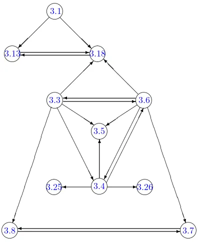
u′=u, v′ = 1 The graph of the substitutions is very cumbersome, therefore we show the most interesting subgraph only.
Fig. 1. A subgraph of the differential substitutions.
Comments. (1) System (3.1) coincides with (1.2) and (3.3) coincides with (1.3).
(2) It was simpler to obtain some systems from (3.6) than (3.3) or vice versa. These systems are connected by the second order invertible substitution, see (3.6) → (3.3) and (3.3) → (3.6). Hence, each system obtained from (3.6) can be obtained from (3.3) and vice versa. (3) Fifteen systems (3.9)–(3.15), (3.18), (3.22), (3.33)–(3.36), (3.38) and (3.40) can be obtained from both (3.1) and (3.6) by the presented differential substitutions. Twelve systems (3.2), (3.16), (3.17), (3.23), (3.24), (3.27)–(3.30), (3.32), (3.37) and (3.39) can be obtained from (3.1). The remaining eleven systems (3.3)–(3.5), (3.7), (3.8), (3.19)–(3.21), (3.25), (3.26) and (3.31) can be obtained from (3.6) or (3.3).
Remark 7. As the systems (3.1) and (3.3) have the Lax representations, then all systems from the list have the Lax representations in a generalized meaning (see Section 5).
Remark 8. Some of the presented substitutions are superpositions of lower order substitutions, other substitutions are irreducible.
either. Systems (3.4) and (3.6) admit the substitutions from the first till fourth orders. We do not present higher order substitutions for (3.4) because simpler substitutions exist for (3.6). Fifth and higher order substitutions for systems (3.4) and (3.6) have not been computed because the computations are extremely cumbersome.
Remark 10. There are some additional differential substitutions under the constraints for constants in the systems. For example, there are substitutions (3.1) → (3.31) for c1 = 0 and (3.6)→(3.32) for c3 = 0 or (3.6)→(3.39) for c2= 0 and so on. These substitutions are not so important and we do not present them here.
Remark 11. Unexpectedly, the well known systems (3.1) and (3.3) are implicitly connected as it is shown in Fig. 1.
5
Examples of zero curvature representations
The IST method for nonlinear equations with two independent variables is based on investigation of a linear overdetermined system
L(u, λ, ∂x)ψ= 0, ψt=A(u, λ, ∂x)ψ, (5.1)
where Land A are ordinary linear operators, uis a smooth (vector) function satisfying a
non-linear partial differential equation E(u) = 0 andλis a parameter. The operatorsL, Amay be
both scalar and matrix. The operators L,A and E may be also pseudodifferential or integro-differential. The compatibility condition of system (5.1) reads
∂L ∂t +LA
ψ
Lψ=0 = 0.
There are two ways to satisfy this condition. The first operator condition was introduced by P.D. Lax [37]:
∂L
∂t +LA=AL, or
∂L
∂t = [A, L]. (5.2)
The second more general operator condition was introduced in [38], see also [39]:
∂L
∂t +LA=BL. (5.3)
If an equation E(u) = 0 is equivalent to equation (5.2), then (5.2) is said to be the Lax
representation of the equation E(u) = 0. The pair of operators (L, A) is said to be the (L, A
)-pair or the Lax )-pair.
If an equationE(u) = 0 is equivalent to equation (5.3), then (5.3) is said to be the (L, A, B)
representation of the equation E(u) = 0 or the triad representation.
In all cases, operatorLmust essentially depend on the parameterλ. This parameter cannot be removed by a gauge transformation L→f−1Lf with some smooth functionf, in particular. If system (5.1) is differential, then the standard substitution ψ = Ψ1, ψx = Ψ2 and so on, provides the following first order system:
Ψx=UΨ, Ψt=VΨ, (5.4)
whereU andV are square matrices depending onuandλ. The compatibility condition of linear
system (5.4) reads
if E(u) = 0. Usually a stronger condition is required: (5.5) is valid iff E(u) = 0. In this
case equation (5.5) is said to be the zero curvature representation. For an evolutionary system
ut =K(u,ux, . . . ,un), u ={uα} the matrix U usually depend onu only, but it may depend
on u,ux,uxx, and so on. Let us consider the general case.
If some smooth functions F =F(u,ux, . . . ,ur) and Φ = Φ(u,ux, . . . ,up) satisfy the
condi-tion
∂tF+ Φ ut=K
= 0, (5.6)
then one obtains
Φ ut=K
= Φ, ∂tF ut=K
= ∂F
∂uαi ∂tu
α i
ut=K = ∂F
∂uαi ∂
i xuαt
ut=K = ∂F
∂uαi D
i xKα,
where the summation overi= 0, . . . , r and α= 1, . . . , mis implied. This implies
Φ =−∂F
∂uαi D
i xKα
according to (5.6). Using this result one obtains the following identity:
∂tF + Φ≡
∂F ∂uα
i
Dix(uαt −Kα), ∀u (5.7)
for anyF and Φ satisfying (5.6).
Let us apply identity (5.7) to equation (5.5). If the matrixU depends onuonly then
Ut−Vx+ [U, V] =
∂U ∂uα(u
α
t −Kα), ∀u. (5.8)
It is obvious now that equation (5.5) is equivalent to ut = K iff the matrices ∂U/∂uα, α =
1, . . . , m are linearly independent. Suppose now that the matrix U depends on u and ux then
one obtains
Ut−Vx+ [U, V] =
∂U ∂uα(u
α
t −Kα) +
∂U ∂uα
x
Dx(uαt −Kα), ∀u. (5.9)
If the matrices∂U/∂uα,∂U/∂uβ
x,α, β= 1, . . . , mare linearly independent, then equation (5.5) is equivalent tout=K again. Otherwise, equation (5.5) would be equivalent to some differential
consequence of the system ut=K that is a more general system than the original one. In this
case we call equation (5.5) thegeneralized zero curvature representation.
It is well known that equations (5.4) and (5.5) are covariant under the following transforma-tion
¯
Ψ =S−1Ψ, U¯ =S−1(U S−Sx), V¯ =S−1(V S−St), (5.10)
where S is any non-degenerate matrix. This transformation is called a gauge one. Any gauge transformation is invertible and preserves compatibility of system (5.4).
Two (L, A)-pairs were proposed for system (1.2) in [3]. One of these (L, A)-pairs coincides with the (L, A)-pair that was presented in [4]. The L-operator of the common (L, A)-pair takes the form L= (∂x2+f)(∂x2−g), where
The temporal Lax equation reads ψt = Aψ, where A is a fractional degree of L. The spatial Lax equation Lψ =λ2ψ can be transformed into the system (∂2
x−g)ψ=λϕ, (∂x2+f)ϕ=λψ and then into the normal form (5.4), were
U =
Here f1 andf2 take the following form:
f1 = 181(3v2−2u2+ 2v2)−2λ2, f2= √
2
18(3u2+uv).
Matrices (5.11) realize the zero curvature representation of system (1.2).
System (1.3) also has two Lax representations (see [3]). Using the simpler L-operator, we have found, similarly to the previous case, the following matrices that realize the zero curvature representation of system (1.3):
˜
where
h1= 14(u1−v1)2, h2 = 14(u1+v1)2.
One can easily verify that matrices A= ˆUu2 and B = ˆUv2 are commutative, hence the system
Sx = (Auxx +Bvxx)S has the following solution S = exp(Aux+Bvx). The matrix U1 = U¯ˆ evaluated according to (5.10) takes the following form
U1 =
Now another gauge transformation is possible with the following diagonal matrix:
S1 = exp Z
diag (U1)dx
,
where diag (U1) is the main diagonal of U1. This gauge transformation provides the following matrix
A correspondingV-matrix can be obtained by solving equation (5.5) directly or by the previous twofold gauge transformation. This matrix takes the following form
V2=
The matricesU2 and V2 realize the zero curvature representation of system (3.9). B.Substitution (3.1)→ (3.17) reduces matrixU from (5.11) to the following form formation. It is clear from the structure of the matrix ˆU that
whereAandBare some linearly independent matrices. Thus, this zero curvature representation for system (3.17) is generalized. Of course, one may introduce here the new variable u′ =u
1 to obtain an ordinary zero curvature representation. But we do not know if it is always possible.
C.Performing the substitution (3.3) → (3.6) into the matrix U from (5.12) one obtains
The result of the twofold gauge transformation is
˜
Matrices ˜U2 and ˜V2 realize the zero curvature representation of system (3.6).
6
Conclusion
representations are obtained from the Drinfeld–Sokolov L,A operators by using corresponding differential substitutions listed in Section 4. Matrices U and V that realize all zero curvature representations have the size 4×4. Thus, the two-field evolutionary systems presented above are integrable in principle by the inverse spectral transform method. But the fact is that the inverse scattering problem for differential equations with order more than two is extremely difficult. That is why other methods for solution of equations may be useful [40]. They may be B¨acklund transformations [41], Darboux transformations [42,43], Hirota method [44] or numeric simulating (see [45], for example).
Acknowledgments
We are grateful to Professor V.V. Sokolov for helpful discussions. This work was supported by Federal Agency for Education of Russian Federation, project # 1.5.07.
References
[1] Ablowitz M.J., Segur M., Solitons and the inverse scattering transform, SIAM, Philadelphia, 1981.
[2] Zakharov V.E., Manakov S.V., Novikov S.P., Pitaevsky L.P., Theory of solitons: inverse problem method, Nauka, Moscow, 1980.
[3] Drinfeld V.G., Sokolov V.V., New evolution equations having(L-A)pairs,Trudy Sem. S.L. Soboleva, Inst.
Mat., Novosibirsk2(1981), 5–9 (in Russian).
[4] Hirota R., Satsuma J., Soliton solutions of a coupled Korteweg–de Vries equation,Phys. Lett. A85(1981), 407–408.
[5] Antonowicz M., Fordy A., Coupled KdV equations with multi-Hamiltonian structures,Phys. D28(1987),
345–357.
[6] Ma W.-X. A class of coupled KdV systems and their bi-Hamiltonian formulation,J. Phys. A: Math. Gen.
31(1998), 7585–7591,solv-int/9803009.
[7] Ma W.-X., Pavlov M., Extending Hamiltonian operators to get bi-Hamiltonian of coupled KdV systems,
Phys. Lett. A246(1998), 511–522,solv-int/9807002.
[8] Fuchssteiner B., The Lie algebra structure of degenerate Hamiltonian and bi-Hamiltonian systems,Progr.
Theoret. Phys.68(1982), 1082–1104.
[9] Nutku Y., Oˇguz ¨O., Bi-Hamiltonian structure of a pair of coupled KdV equations, Nuovo Cimento 105
(1990), 1381–1383.
[10] Gerdt V.P., Zharkov A.Y., Computer classification of integrable coupled KdV-like systems, J. Symbolic
Comput.10(1990), 203–207.
[11] Foursov M.V., On integrable coupled KdV-type systems,Inverse Problems16(2000), 259–274.
[12] Zharkov A.Y., Computer classification of the integrable coupled KdV-like systems with unit main matrix,
J. Symbolic Comput.15(1993), 85–90.
[13] Karasu A., Painlev´e classification of coupled Korteweg–de Vries-type systems, J. Math. Phys. 38(1997),
3616–3622.
[14] Foursov M.V., Towards the complete classification of homogeneous two-component integrable equations,
J. Math. Phys.44(2003), 3088–3096.
[15] Meshkov A.G., Sokolov V.V., Integrable evolution equations on the N-dimensional sphere, Comm. Math.
Phys.232(2002), 1–18.
[16] Meshkov A.G., Sokolov V.V., Classification of integrable divergentN-component evolution systems,Theoret. and Math. Phys.139(2004), 609–622.
[17] Balakhnev M.Ju., A class of integrable evolutionary vector equations.Theoret. and Math. Phys.142(2005), 8–14.
[18] Balakhnev M.Ju., Meshkov A.G., Integrable anisotropic evolution equations on a sphere,SIGMA1(2005),
027, 11 pages,nlin.SI/0512032.
[20] Kulemin I.V., Meshkov A.G., To the classification of integrable systems in 1+1 dimensions, in Proceedings Second International Conference “Symmetry in Nonlinear Mathematical Physics” (July 7–13, 1997, Kyiv), Editors M. Shkil, A. Nikitin and V. Boyko, Institute of Mathematics, Kyiv, 1997, 115–121.
[21] Meshkov A.G., On symmetry classification classification of third order evolutionary systems of divergent type,Fundam. Prikl. Mat.12(2006), no. 7, 141–161 (in Russian).
[22] Ibragimov N.Kh., Shabat A.B., On infinite Lie–B¨acklund algebras,Funktsional. Anal. i Prilozhen.14(1980), no. 4, 79–80 (in Russian).
[23] Svinolupov S.I., Sokolov V.V., Evolution equations with nontrivial conservation laws, Funktsional. Anal. i Prilozhen.16(1982), no. 4, 86–87.
[24] Sokolov V.V., Shabat A.B., Classification of integrable evolution equations,Soviet Scientific Reviews, Sec-tion C4(1984), 221–280.
[25] Mikhailov A.V., Shabat A.B., Yamilov R.I., The symmetry approach to the classification of integrable equations. Complete lists of integrable systems,Russian Math. Surveys42(1987), no. 4, 1–63.
[26] Mikhailov A.V., Shabat A.B., Sokolov V.V., The symmetry approach to the classification of integrable equations, in Integrability and Kinetic Equations for Solitons, Editors V.G. Bahtariar, V.E. Zakharov and V.M. Chernousenko, Naukova Dumka, Kyiv, 1990, 213–279 (English transl.: in What is Integrability?, Springer-Verlag, New York, 1991, 115–184).
[27] Fokas A.S., Symmetries and integrability,Stud. Appl. Math.77(1987), 253–299.
[28] Galindo A., Martinez L., Kernels and ranges in the variational formalism, Lett. Math. Phys. 2 (1978),
385–390.
[29] Drinfeld V.G., Sokolov V.V., Lie algebras and equations of Korteweg–de Vries type, Current Problems in
Mathematics, Vol. 24, Itogi Nauki i Tekhniki, VINITI, Moscow, 1984, 81–180 (English transl.: J. Sov. Math.
30(1985), 1975–2035).
[30] Balakhnev M.Yu., Kulemin I.V., Differential substitutions for third-order evolution systems,Differ. Uravn. Protsessy Upr.(2002), no. 1, 7 pages (in Russian), available athttp://www.neva.ru/journal/j/.
[31] Zakharov V.E., Shabat A.B., Exact theory of two-dimensional focusing and one-dimensional self-modulation of waves in nonlinear media,Z. Eksper. Teoret. Fiz.ˇ 61(1971), no. 1, 118–134 (English transl.:
Soviet Physics JETP34(1972), no. 1, 62–69).
[32] Chen H.H., Lee Y.C., Liu C.S., Integrability of nonlinear Hamiltonian systems by inverse scattering method,
Phys. Scripta20(1979), 490–492.
[33] Meshkov A.G., Necessary conditions of the integrability,Inverse Problems10(1994), 635–653.
[34] Fuchssteiner B., Fokas A.S., Symplectic structures, their B¨acklund transformations and hereditary symme-tries,Phys. D4(1981/82), 47–66.
[35] Drinfeld V.G., Sokolov V.V., Equations that are related to the Korteweg–de Vries equation, Dokl. Akad.
Nauk SSSR284(1985), no. 1, 29–33 (in Russian).
[36] Meshkov A.G., Tools for symmetry analysis of PDEs,Differ. Uravn. Protsessy Upr.(2002), no. 1, 53 pages,
available athttp://www.neva.ru/journal/j/.
[37] Lax P.D., Integrals of nonlinear equations of evolution and solitary waves, Comm. Pure Appl. Math. 21
(1968), 467–490.
[38] Manakov S.V., The method of the inverse scattering problem, and two-dimensional evolution equations,
Uspehi Mat. Nauk31(1976), no. 5, 245–246 (in Russian).
[39] Zakharov V.E., Inverse scattering method, in Solitons, Editors R.K. Bullough and P.J. Caudrey, Springer-Verlag, New York, 1980, 270–309.
[40] Dodd R.K., Eilbeck J.C., Gibbon J.D., Morris H.C., Solitons and nonlinear wave equations, Academic Press Inc., London, 1984.
[41] Miura R.M. (Editors), B¨acklund transformations, the inverse scattering method, solitons, and their
appli-cations, NSF Research Workshop on Contact Transformations, Lecture Notes in Mathematics, Vol. 515,
1976.
[42] Matveev V.B., Salle M.A., Darboux transformations and solitons, Springer, Berlin, 1991.
[43] Gu C.H., Hu H.S., Zhou Z.X., Darboux transformations in soliton theory and its geometric applications, Shanghai Scientific and Technical Publishers, Shanghai, 1999.
[44] Hirota R., The direct method in soliton theory, Cambridge University Press, Cambridge, 2004.