Estimating the Technology of
Cognitive and Noncognitive Skill
Formation
Flavio Cunha
James J. Heckman
a b s t r a c t
This paper estimates models of the evolution of cognitive and noncognitive skills and explores the role of family environments in shaping these skills at different stages of the life cycle of the child. Central to this analysis is identification of the technology of skill formation. We estimate a dynamic factor model to solve the problem of endogeneity of inputs and multiplicity of inputs relative to instruments. We identify the scale of the factors by estimating their effects on adult outcomes. In this fashion we avoid reliance on test scores and changes in test scores that have no natural metric. Parental investments are generally more effective in raising noncognitive skills. Noncognitive skills promote the formation of cognitive skills but, in most specifications of our model, cognitive skills do not promote the formation of noncognitive skills. Parental inputs have different effects at different stages of the child’s life cycle with cognitive skills affected more at early ages and noncognitive skills affected more at later ages.
Flavio Cunha is an assistant professor of economics at the University of Pennsylvania. James J Heckman is a professor of economics at the University of Chicago, American Bar Foundation and University College Dublin. This research was supported by NIH R01-HD043411, NSF SES-024158, the Committee for Economic Development with a grant from the Pew Charitable Trusts and the Partnership for America’s Economic Success, and the J.B. Pritzker Consortium on Early Childhood Development at the Harris School of Public Policy, University of Chicago. Flavio Cunha also acknowledges support from the Claudio Haddad dissertation fund at the University of Chicago and Dr. Rob Dugger. The views expressed in this paper are those of the authors and not necessarily those of the funders listed here. The first draft of this paper was presented at a conference at the Minneapolis Federal Reserve, October 2003. The authors received helpful comments from Robert Pollak at a seminar at Washington University, February 2004, from Susanne Schennach who is a coauthor of a successor paper, Petra Todd, and Kenneth Wolpin. They also received helpful comments from the editor and three anonymous referees. A website containing supplementary material is available at http://jenni.uchicago.edu/idest-tech. The data used in this article can be obtained beginning May 2009 through April 2012 from James J. Heckman, University of Chicago, Department of Economics, 1126 E. 59thStreet, Chicago IL 60637;
jjh@uchicago.edu.
½Submitted May 2006; accepted December 2006
ISSN 022-166X E-ISSN 1548-8004Ó2008 by the Board of Regents of the University of Wisconsin System
I. Introduction
The importance of cognitive skills in explaining socioeconomic suc-cess is now firmly established. An emerging body of empirical research documents the importance of noncognitive skills for predicting wages, schooling, and participa-tion in risky behaviors.1Heckman, Stixrud, and Urzua (2006) demonstrate that cog-nitive and noncogcog-nitive skills are equally important in explaining a variety of aspects of social and economic life in the sense that movements from the bottom to the top of the noncognitive and cognitive distributions have comparable effects on many out-comes.
There is a substantial body of empirical research on the determinants of cognitive test scores and their growth.2 There is no previous research on the determinants of the evolution of noncognitive skills. This paper identifies and estimates models of the technology of skill formation. Building on the theoretical analyses of Cunha and Heckman (2007) and Cunha, Heckman, Lochner, and Masterov (2006), we esti-mate the joint evolution of cognitive and noncognitive skills over the life cycle of children.
We model the self productivity of skills as well as their dynamic complementarity. Our technology formalizes the notion that noncognitive skills foster acquisition of cognitive skills by making children more adventuresome and open to learning.3 It also formalizes the notion that cognitive skills can promote the formation of noncog-nitive skills. With our estimated technology, it is possible to define and measure crit-ical and sensitive periods in the life cycle of child development, and to determine at which ages inputs most affect the evolution of skills.
Psychologists who study child development have long advocated the importance of understanding the formation of noncognitive skills for interpreting the effects of early childhood intervention programs (see Raver and Zigler 1997; Zigler and Butterfield 1968). Heckman, Stixrud, and Urzua (2006) note that the Perry Preschool Program did not raise IQ, but promoted success among its participants in a variety of aspects of social and economic life. Our analysis of noncognitive skills, their role in shaping cognitive skills, our investigation of the role of cognitive skills in shaping noncognitive skills, and our determination of the effectiveness of parental inputs on the formation of both types of skill over the life cycle, are first steps toward pro-viding a unified treatment of the early intervention and family influence literatures. The conventional approach to estimating cognitive production functions is best ex-emplified by the research of Todd and Wolpin (2003; 2005). A central problem with the production function approach is accounting for the endogeneity of inputs. An-other problem is the wealth of candidate parental input measures available in many data sets. The confluence of these two problems—endogeneity and the multiplicity
1. See Bowles, Gintis, and Osborne (2001), Heckman and Rubinstein (2001), and Heckman, Stixrud, and Urzua (2006).
2. Todd and Wolpin (2003) survey the educational production function literature as well as the child de-velopment literature.
of input measures—places great demands on standard instrumental variable (IV) and fixed effect procedures, such as those used by Todd and Wolpin. It is common in studies of cognitive production functions for analysts to have more inputs than instru-ments. Indices of inputs are used to circumvent this problem and reduce the parental input data to more manageable dimensions. The constructed indices often have an ad hoc quality about them and may be poor proxies for the true combination of inputs that enter the technology.
Our approach to the identification of the technology of skill formation bypasses these problems. We estimate a dynamic factor model that exploits cross-equation restrictions (covariance restrictions in linear systems) to secure identification using a version of dynamic state space models (Shumway and Stoffer 1982; Watson and Engle 1983). The idea underlying our approach is to model cognitive and noncogni-tive skills, as well as parental investments as low dimensional latent variables. Build-ing on the analyses of Jo¨reskog and Goldberger (1975), Jo¨reskog, So¨rbom, and Magidson (1979), Bollen (1989) and Carneiro, Hansen, and Heckman (2003), we use a variety of measurements related to skills and investments to proxy latent skills and investments. With enough measurements relative to the number of latent skills and investments, we can identify the latent state space dynamics generating the evo-lution of skills through cross-equation restrictions. When instruments are required, they are internally justified by the model of Cunha and Heckman (2007). We econ-omize on the instruments required to secure identification, which are often scarce. We solve the problem of the multiplicity of measures of parental investments by us-ing all of them as proxies for low dimensional latent investments. Instead of creatus-ing an arbitrary index of parental inputs, we estimate an index that best predicts latent skill dynamics.
We also address a recurring problem in the literature on cognitive production func-tions. Studies in this tradition typically use a test score as a measure of output (see, for example, Hanushek 2003). Yet test scores are arbitrarily normalized. Any mono-tonic transformation of a test score is also a valid test score. Value added—the change in test scores over stages (or grades)—is not invariant to monotonic transfor-mations.
We solve the problem of defining a scale for output by anchoring our test scores using the adult earnings of the child, which have a well-defined cardinal scale. Other anchors such as high school graduation, college enrollment, and the like could also be used. Thus, we anchor the scale of the latent factors that generate test scores by determining how the factors predict adult outcomes.4This sets the scale of the test scores and factors in an interpretable metric.
Applying our methodology to CNLSY data we find that: (1) Both cognitive and noncognitive skills change over the life cycle of the child. (2) Parental inputs affect the formation of both noncognitive skills and cognitive skills. Direct measures of mothers’ ability affect the formation of cognitive skills but not noncognitive skills. (3) Parental inputs appear to affect cognitive skill formation more strongly at earlier ages. They affect noncognitive skill formation more strongly at later ages. Ages where parental inputs have higher marginal productivity, holding all inputs constant,
are called ‘‘sensitive’’ periods. The sensitive periods for cognitive skills occur earlier in the life cycle of the child than do sensitive periods for noncognitive skills. Our evidence is consistent with the evidence presented in Carneiro and Heckman (2003) that noncognitive skills are more malleable at later ages than cognitive skills. See also the evidence in Heckman (2007) and in Borghans et al. (2008). We also find that (4) measurement error in inputs is substantial and that correcting for measure-ment error greatly affects our estimates.
The plan of this paper is as follows. Section II briefly summarizes our previous research on models of skill formation. Section III presents our analysis of identifica-tion using dynamic factor models. Secidentifica-tion IV discusses our empirical findings. Secidentifica-tion V concludes. We use a technical appendix to present our likelihood function. A web-site provides supporting material.5
II. A Model of Cognitive and Noncognitive
Skill Formation
Cunha and Heckman (2007) analyze multiperiod models of child-hood skill formation followed by a period of adultchild-hood.6 They extend the model of Becker and Tomes (1986), who assume childhood lasts one period, and that invest-ment inputs at different stages of the life cycle of a child are perfect substitutes and are equally productive. Becker and Tomes do not distinguish cognitive from noncog-nitive skills. Cunha and Heckman (2007) analyze models with two kinds of skills:uC
anduN
, whereuC
is cognitive skill anduN
is noncognitive skill. LetuI
k;t denote parental investments in child skillk in periodt,k2 fC;Ngand
t2 f1;.;Tg, where Tis the number of periods of childhood. Leth be the level
of human capital as the child starts adulthood which depends on both uC
T+1 and
uN
T+1. The parents fully control the investment in the child. A better model would
in-corporate investment decisions of the child as influenced by the parent through the process of preference formation, and through parental incentives for influencing child behavior. We leave the development of that model for another occasion.
Assume that each agent is born with initial conditionsu#1¼ uC
1;uN1
. Family en-vironmental and genetic factors may influence these initial conditions (see Olds 2002 and Levitt 2003). At each stagetletu#t ¼ uCt;uNt
denote the 132 vector of skill or ability stocks. The technology of production of skillkin periodtis
uk t+1¼f
k tðut;uIk;tÞ ð1Þ
fork2 fC;Ngandt2 f1;.;Tg.7In this model, stocks of both skills and abilities
produce next period skills and influence the productivity of investments. Cognitive skills can promote the formation of noncognitive skills and vice versa because ut
is an argument of Equation 1. Cunha and Heckman (2007) summarize the evidence
5. See http://jenni.uchicago.edu/idest-tech.
6. See also their web appendix, where more general models of skill formation are analyzed. 7. We assume thatfk
t is twice continuously differentiable, increasing and concave inu I
in economics and psychology about the interaction between cognitive and noncogni-tive skills in the production of human capital.
Adult human capitalhis a combination of periodT+ 1 skills accumulated by the end of childhood:
h¼g uC T+1;uNT+1
:
ð2Þ
The functiongis assumed to be continuously differentiable and increasing inuC T+1
anduN
T+1. This specification of human capital assumes that there is no comparative
advantage in the labor market or in other areas of social performance.8
Early stocks of abilities and skills promote later skill acquisition by making later investment more productive. Students with greater early cognitive and noncognitive abilities are more efficient in later learning of both cognitive and noncognitive skills. The evidence from the early intervention literature suggests that the enriched early environments of the Abecedarian, Perry, and Child-Parent Center programs promote greater efficiency in learning in schools and reduce problem behaviors. See Blau and Currie (2006), Cunha and Heckman (2007), Cunha et al. (2006), and Heckman, Stix-rud, and Urzua (2006).
Technology 1 is sufficiently rich to capture the evidence on learning in rodents and macaque monkeys documented by Meaney (2001) and Cameron (2004) respectively. See Knudsen et al. (2006) for a review of the literature. Emotionally nurturing early environments producing motivation and self-discipline create preconditions for later cognitive learning. More emotionally secure young animals explore their environments more actively and learn more quickly. This is an instance of dynamic complementarity. Using Technology 1, Cunha and Heckman (2007) define critical and sensitive peri-ods for investment. At some ages, and for certain skills, parental investment may be more productive than in other periods. Such periods are ‘‘sensitive’’ periods. If invest-ment is productive only in a single period, it is a ‘‘critical’’ period for that investinvest-ment. Cunha and Heckman (2007) discuss the role of complementarity in investments. If early investments are complementary with later investments, then low early in-vestments, associated with disadvantaged childhoods, make later investments less productive. High early investments have a multiplier effect in making later invest-ments more productive. If investment inputs are not perfect substitutes but are instead complements, government investment in the early years for disadvantaged children promotes investment in the later years.
Cunha and Heckman (2007) show that there is no tradeoff between equity and efficiency in early childhood investments. Government policies to promote early ac-cumulation of human capital should be targeted to the children of poor families. However, the optimal later period interventions for a child from a disadvantaged en-vironment depend critically on the nature of the technology of skill production. If
8. Thus we rule out one potentially important avenue of compensation that agents can specialize in tasks that do not require the skills in which they are deficient. Borghans, ter Weel, and Weinberg (2007b) discuss evidence against this assumption. Cunha, Heckman, Lochner, and Masterov (2006) present a more general task function that captures the notion that different tasks require different combinations of skills and abil-ities. If we assume that the output (reward) in adult taskjisgj uCT+1;uNT+1;h
, wherehis a person-specific parameter and there areJdistinct tasks, we can definegˆjuCT+1;u
N T+1;h
¼max j gj u
C T+1;u
N T+1;h
J
j¼1and
early and late investments are perfect complements, on efficiency grounds a low early investment should be followed up by low later investments.
If inputs are perfect substitutes, later interventions can, in principle, eliminate ini-tial skill deficits. At a sufficiently high level of later-period investment, it is techni-cally possible to offset low initial investments. However, it may not be cost effective to do so. Cunha and Heckman (2007) give exact conditions for no investment to be an efficient outcome in this case. Under those conditions, it would be more efficient to give children bonds that earn interest, rather than invest in their human capital in order to raise their incomes.
The key to understanding optimal investment in children is to understand the tech-nology and market environment in which agents operate. This paper focuses on iden-tifying and estimating the technology of skill formation, which is a vital ingredient for designing skill formation policies, and evaluating their performance.
III. Identifying the Technology using Dynamic
Factor Models
Identifying and estimating Technology 1 is a challenging task. Both the inputs and outputs can only be proxied, and measurement error is likely to be a serious problem. In addition, the inputs are endogenous because parents choose them.
General nonlinear specifications of Technology 1 raise additional problems regard-ing measurement error in latent variables in nonlinear systems (see Schennach 2004). This paper estimates linear specifications of Technology 1. A more general nonlinear analysis requires addressing additional econometric and computational considera-tions, which are addressed in Cunha, Heckman, and Schennach (2007).
A. Identifying Linear Technology
Using a linear specification, we can identify critical and sensitive periods for inputs. We can also identify cross-effects, as well as self-productivity of the stocks of skills. If we find little evidence of self-productivity, sensitive or critical periods, or cross-effects in a simpler setting, it is unlikely that a more general nonlinear model will overturn these results. Identifying a linear technology raises many challenges that we address in this paper.
There is a large body of research that estimates the determinants of the evolution of cognitive skills. Todd and Wolpin (2003) survey this literature. To our knowledge, there is no previous research on estimating the evolution of noncognitive skills.
The empirical analysis reported in Todd and Wolpin (2005) represents the state of the art in modeling the determinants of the evolution of cognitive skills.9In their pa-per, they use a scalar measure of cognitive ability uC
t+1
in periodt+ 1 that depends on periodtcognitive ability uC
t
and investment. We denote investment byuI tin this
and remaining sections, rather thanuI
k;t, as in the preceding section. This notation
reflects the fact that we cannot empirically distinguish between investment in cogni-tive skills and investment in noncognicogni-tive skills. Todd and Wolpin assume a linear-in-parameters technology
uC
t+1¼atuCt +btuIt+ht; ð3Þ
wherehtrepresents unobserved inputs, measurement error, or both. They allow inputs
to have different effects at different stages of the child’s life cycle. They use the com-ponents of the ‘‘home score’’ measure to proxy parental investment.10We use a version of the inputs into the home score as well, but in a different way than they do.
Todd and Wolpin (2003; 2005) discuss problems arising from endogenous inputs
uC t;u
I t
that depend on unobservableht. In their 2005 paper, they use IV methods
coupled with fixed effect methods.11Reliance on IV is problematic because of the ever-present controversy about the validity of exclusion restrictions. As stressed by Todd and Wolpin, fixed effect methods require very special assumptions about the nature of the unobservables, their persistence over time and the structure of agent de-cision rules.12The CNLSY data used by Todd and Wolpin (2005) and in this paper have a multiplicity of investment measures subsumed in a ‘‘home score’’ measure which combines many diverse parental input measures into a score that weights all components equally.13As we note below, use of arbitrary aggregates calls into question the validity of instrumental variable estimation strategies for inputs.
Todd and Wolpin (2005) and the large literature they cite use a cognitive test score as a measure of output. This imparts a certain arbitrariness to their analysis. Test scores are arbitrarily normed. Any monotonic function of a test score is a perfectly good alternative test score. A test score is only a relative rank. While Todd and Wol-pin use raw scores and others use ranks (see, for example, Carneiro and Heckman 2003; and Carneiro, Heckman, and Masterov 2005), none of these measures is intrin-sically satisfactory because there is no meaningful cardinal scale for test scores.
We address this problem in this paper by using adult outcomes to anchor the scale of the test score. Cunha, Heckman, and Schennach (2007) address this problem in a more general way for arbitrary monotonically increasing transformations of the fac-tors. In this paper, we develop an interpretable scale for uC
t;u N
t that is robust to all
affine transformations of the units in which factors uC t;uNt
are measured. For exam-ple, using adult earningsYas the anchor, we write
lnY¼m+dCuC T+1+d
NuN T+1+e;
ð4Þ
where the scales ofuC
T+1andu
N
T+1are unknown. For any affine transformation ofu
k T+1,
corresponding to different units of measuring the factors, the value ofdk
and the in-tercept adjust and we can uniquely identify the left-hand side of
10. This measure originates in the work of Bradley and Caldwell (1980; 1984) and is discussed further in Section IV.
11. See Hsiao (1986); Baltagi (1995); and Arellano (2003) for descriptions of these procedures. 12. Fixed effect methods do not easily generalize to the nonlinear frameworks that are suggested by our analysis of the technology of skill formation. See, however, the analysis of Altonji and Matzkin (2005) for one approach to fixed effects in nonlinear systems.
@lnY
t. Thus, although the scale ofd k
is not uniquely determined, nor is the scale ofuk
T+1, the scale ofd
kuk
T+1is uniquely determined by its effect on log earnings and
we can define the effects of all inputs on lnYrelative to their effects on earnings. The scale for measuring investmentuI
t is also arbitrary. We report results for
alter-native normalizations of the units of investment. Natural scales are in dollars or log dollars. Using elasticities,
produces parameters that are invariant to linear transformations of the units in which investment is measured. This approach generalizes to multiple factors and multiple anchors and we apply it in this paper. We now develop our empirical approach to identifying and estimating the technology of skill formation.
B. Estimating the Technology of Production of Cognitive and Noncognitive Skills
Our analysis departs from that of Todd and Wolpin (2005) in six ways. (1) We analyze the evolution of both cognitive and noncognitive outcomes using the equation system
uN
. We determine how stocks of cognitive and noncognitive skills at datetaffect the stocks at datet+1, examining both self productivity (the effects ofuN
t onu
t+1) and
cross-productiv-ity (the effects ofuC
by vectors of measurements on skills and investments which can include test scores as well as outcome measures.14In our analysis, test scores and parental inputs are indicators of the latent skills and latent investments. We account for measurement errors in output and input variables. We find substantial measurement errors in the proxies for parental investment and in the proxies for cognitive and noncognitive skills. (4) Instead of imposing a particular index of parental input based on compo-nents of the home score, we estimate an index that best fits the data. (5) Instead of relying solely on exclusion restrictions to generate instruments to correct for mea-surement error in the proxies forut, and for endogeneity, we use covariance
restric-tions that exploit a feature of our data that there are many more measurements onut+1
and ut than the number of latent factors. This allows us to secure identification
from cross-equation restrictions using multiple indicator-multiple cause (MIMIC)
(Jo¨reskog and Goldberger 1975) and linear structural relationship (LISREL) (Jo¨re-skog, So¨rbom, and Magidson 1979) models.15When instruments are needed, they arise from the internal logic of the model developed in Cunha et al. (2006) and Cunha and Heckman (2007), using methods developed by Madansky (1964) and Pudney (1982). (6) Instead of relying on test scores as measures of output and change in output due to parental investments, we anchor the scale of the test scores using adult outcome measures: log earnings and the probability of high school graduation. We thus estimate the effect of parental investments on the adult earnings of the child and on the probability of high school graduation.
C. Model for the Measurements
We assume access to measurement systems that can be represented by a dynamic fac-tor structure:
Yjk;t¼mk j;t+a
k j;tu
k t+e
k
j;t;forj2 f1;.;m k
tg;k2 fC;N;Ig;
wheremk
t is the number of measurements on cognitive skills, noncognitive skills, and
investments in period t; and where uk
t is a dynamic factor for component k,
k 2 fC;N;Ig. Varðek
j;tÞ ¼s2k;j;t. We account for latent initial conditions of the
pro-cess, uC
1;uN1
, which correspond to endowment of abilities. Because we have mul-tiple measurements of abilities in the first period of our data, we can also identify the distribution of the latent initial conditions. We also identify the distribution of each
ut¼ uCt;uNt;uIt
, as well as the dependence acrossutandut#;t6¼t#. Themkj;tand the
ak
j;tcan depend on regressors which we keep implicit.
As above, letuC
t denote the stock of cognitive skill of the agent in periodt. We do
not observeuC
t directly. Instead, we observe a vector of measurements, such as test
scores,YC
j;t, forj2 f1;2;.;mCtg. Assume that:
YjC;t¼mC j;t+a
C j;tu
C
t +e
C
j;tforj2 f1;2;.;m C tg ð7Þ
and setaC
1;t¼1 for allt. Some normalization is needed to set the scale of the factors.
ThemC
j;t may depend on regressors.
We have a similar equation for noncognitive skills at aget, relatinguN
t to proxies
for it:
YjN;t¼mNj;t+aNj;tuNt +eNj;tforj2 f1;.;mNtg ð8Þ
and we normalizeaN
1;t¼1 for allt. Finally, we model the measurement equations for
investments,uI t:
YI
j;t¼mIj;t+aIj;tutI+eIj;tforj2 f1;.;mItg ð9Þ
and the factor loadingaI
1;t¼1. Thee’s are measurement errors that account for the
fallibility of our measures of latent skills and investments.16Again, themI
j;t andaIj;t
may depend on the regressors which we keep implicit. We analyze a linear law of motion for skills:
uk
where the error termhk
t is independent across agents and over time for the same
agents, buthC
t and hNt are freely correlated. We assume that the htk, k2 fC;Ng,
are independent of uC
1;u
N
1
. Below, we show how to relax the independence assump-tion and allow for unobserved inputs. Thegk
l,l¼0;.;3 may depend on regressors
which we keep implicit.
We allow the components ofutto be freely correlated for anytand with any vector
ut#;t#6¼t, and we can identify this dependence. We assume that any variables in the
mk
j;t are independent ofut,ekj;t, andhkt fork2 fC;N;Igandt2 f1;.;Tg. We now
establish conditions under which the technology parameters are identified.
D. Semiparametric Identification
The goal of the analysis is to recover the joint distribution of uC t;u
tributions of fhk tg
T
t¼1andfekj;tg mk
t
j¼1 nonparametrically, as well as the parameters
fak
of the measurements is straightforward under our assumptions.17
1. Classical Measurement Error for the Case of Two Measurements Per Latent Fac-tor: mCt ¼mNt ¼mIt ¼2
We make the following assumptions about theek j;t:
Assumption 1ek
j;t is mean zero and independent across agents and over time for
t2 f1;.;Tg;j2 f1;2g; andk2 fC;N;Ig;
Assumption 2 ek
j;t is mean zero and independent of u
Assumption 3ek
j;tis mean zero and independent fromeli;t for i;j2 f1;2gand i6¼j
for k¼l; otherwiseek
j;tis mean zero and independent fromeli;tfor i;j2 f1;2g;k6¼l ,
k;l2 fC;N;Igandt2 f1;.;Tg.
16. Measurement Equations 7, 8, and 9 can be interpreted as output-constant demand equations arising from the following two-stage maximization problem. Families use inputs Xj;t with prices Pj,t,
j2 f1;.;mI eral conditions. Specifications (7) - (9) are consistent with Cobb-Douglas and Leontief technologies, when
uI
tis measured in logs. Prices appear in the intercepts. These technologies impose restrictions on the factor loadings of the inputs. See Appendix 1 which develops this point further.
17. Obviously, we cannot separately identify the mean of the factor, Euk t
, and the interceptsmk j;t. It is necessary either to normalize the intercept in one equationmk
1;t¼0 and identify E u k t
, or to normalize Euk
t
a. Identification of the Factor Loadings
t¼1 for every person, we can compute
CovðYk
1;t;Y2l;tÞ from the data for all t,t and k,l pairs, where t;t2 f1;.;Tg;
k;l2 fC;N;Ig. Consider, for example, measurements on cognitive skills. Recall that
aC
1;t¼1. We know the left-hand side of each of the following equations:
Cov Y1C;t;Y1C;t+1
We can identifyaC
2;tby taking the ratio of Equation 12 to Equation 11 andaC2;t+1from
the ratio of Equation 13 to Equation 11. Proceeding in the same fashion, we can iden-tify ak
valid measurements for the factoruk t.
b. The Identification of the Joint Distribution of uC t;u
Once the parametersak
1;tandak2;tare identified (up to the
normaliza-18. The same remark applies as in Footnote 17. We can not separately identify the mean of the factor, Euk
t
, and the interceptsmk
j;t. It is necessary either to normalize the intercept in one equationmk1;t¼0 and identify Euk
mj¼
mC j;t
aC j;t
;m
N j;t
aN j;t
;m
I j;t
aI j;t
!
( )T
t¼1
forj¼1;2:
Letudenote the vector of all factors in all time periods:
u¼ fðuC t;u
N t;u
I tÞg
T t¼1:
We rewrite the measurement equations as
Y1¼m1+u+e1;
Y2¼m2+u+e2:
Under the assumption that measurement error is classical, we can apply Kotlarski’s Theorem (Kotlarski 1967) and identify the joint distribution ofuas well as the dis-tributions ofe1ande2. Sinceak
j;tis identified, it is possible to recover the distribution
ofek
j;tforj2 f1;2;.;mktg;k2 fC;N;Igandt2 f1;2;.;Tg.
Example 1Suppose thatu;N 0ð ;SÞ;ek
j;t;Nð0;sk2;j;tÞ.We observe the vectors Y1
and Y2,m1 and m2 are identified and the Y1 and Y2 can be adjusted accordingly.
As previously established, we can identify the factor loadingsak
j;tby taking the ratio
of covariances such as Equation 12 to 11. To identify the distribution of the factors, we need to identify the variance-covariance matrixS. We can compute the variance of the factoruk
t from the covariance between Y1k;t and Y2k;t :
CovðY1k;t;Y2k;tÞ ¼ak
2;tVarðu k
tÞfork2 fC;N;Ig:
Recall thatak
2;tis identified and the covariance on the left-hand side can be formed
from the data. The covariance of any two elements ofucan be computed from the corresponding moments:
CovðY1k;t;Y1l;tÞ ¼Covðukt;ultÞfork;l2 fC;N;Igandt;t2 f1;.;Tg; ð14Þ
and
CovðYjk;t;Ykl;tÞ ¼ak j;ta
l
k;tCovðukt;u l
tÞ; ð15Þ
where the coefficientsak
j;t;alk;tare known by the previous argument. Since we know VarðYk
j;tÞ;ðakj;tÞandVarðukj;tÞ, we can identifys2k;j;t from these ingredients:
VarðYjk;tÞ2ðakj;tÞ
2
Varðuk
j;tÞ ¼s2k;j;t;k2 fC;N;Ig;t2 f1;.;Tg:
c. The Identification of the Technology Parameters Assuming Independence ofh.
Assume thathk
t is independent of uCt;uNt;uIt
uN
Assume thathN
t is serially independent but possibly correlated withhCt. Define
Y˜N1;t+1¼Y1N;t+12mN
If we estimate Equation 17 by least squares, we do not obtain consistent estimators of
gN
However, we can instrumentY˜N
1;t;Y˜C1;t;Y˜I1;t, usingY2N;t;Y2C;t;Y2I;t as instruments by
applying two-stage least squares to recover the parameters gN
k for k¼1,2,3. See
Madansky (1964) or Pudney (1982) for the precise conditions on the factor loadings. The suggested instruments are also independent ofhN
t because of the assumed lack
of serial correlation inhN t.
19We can repeat the argument for different time periods.
In this way, we can identify stage-specific technologies for each stage of the child’s life cycle. We can perform a parallel analysis for the cognitive skill equation.
2. Nonclassical Measurement Error
We can replace Assumption 3 with the following assumption and still obtain full identification of the model.
Assumption 4 ek
1;t is independent of elj;t for j2 f2;.;mktg;k;l2 fC;N;Ig
The proof of identification is as follows. LetYk j;t¼akj;tu
19. See our website for an analysis of the case in whichhk
CovðY1k;t21;Y1k;tÞ ¼Covðuk
Hence we can identifyak
j;t,j2 f1;.;mktg;t2 f1;.;Tg; andk2 fC;N;Igand thus
since we know every ingredient on the right hand side of the preceding equation. By a similar argument, we can identify
Covðek
j;t;elj#;tÞ ¼CovðYjk;t;Yjl#;tÞ2akj;talj#;tCovðukt;ultÞ: ð19Þ
We can rewrite the measurement equations as a system:
Yjk;t
Applying Schennach (2004), we can identify the joint distribution of ðuC
Example 2 Assume access to three measurements for cognitive, noncognitive, and investment factors, respectively. Suppose that u¼ uC;uN;uI
covariance matrix S is obtained from Equation 14. Furthermore, any element of the matrixVcan be obtained from Equation 19. Finally, we can identifys2
k;j;t from
VarðYk j;tÞ.
For this more general measurement-error system, we can identify stage-specific technologies using the same proof structure as was used for the case with classical measurement error.
3. The Identification of the Technology with Correlated Omitted Inputs
It is unrealistic to assume that omitted inputs are serially independent. Fortunately, we can relax this assumption. Assume now that hk
t is not independent of
u#t¼ ðuC
uN
In this section, we normalizegN
4 ¼1. The termlis a time-invariant input permitted
to be freely correlated withut. We allowlto have a different impact on cognitive
and noncognitive skill accumulation. Letnt¼ ðnNt;nCtÞ. We make the following
as-sumption.
Assumption 5The error termntis independent ofut;l;nt,conditional on
regres-sors for anyt6¼t.
Under this assumption, we can identify both a stage-invariant technology and a stage-varying technology. We first analyze the stage-invariant case. Consider, for ex-ample, the law of motion for noncognitive skills. For any periodst,t+1 we can com-pute the difference
We use the measurement equations to proxy the unobservedu’s:
Y˜N1;t+12Y˜N1;t¼gN
OLS applied to Equation 23 does not produce consistent estimates ofgN
1;gN2, andgN3
because the regressorsðY˜k
1;t2Y˜k1;t21Þare correlated with the error termv, where
However, we can instrument ðY˜k
1;t2Y˜1k;t21Þ using Yjk;t212Yjk;t22
n omkt
j¼2 as
instru-ments. These instruments are valid because of the generalization of investment Equa-tion 9 in Cunha and Heckman (2007) to aTperiod model.20Using a two-stage least squares regression with these instruments allows us to recover the parametersgN
1;gN2
andgN
3. We can identifygN0 if we assume that EðlÞ ¼0. Following a parallel
argu-ment, we can identifygN
0;gN1;gN2 andgN3 using the data on the evolution of cognitive
From the measurement equations, we know the joint distribution of uk
t+1;uNt;uCt;uIt
cN
Under Assumption 5 we can apply Kotlarski’s Theorem to this system and obtain the distribution oflandntfor anyt. Note that we can identify the parametergC4 from the
covariance:
problem raised by correlated omitted inputs for stage-invariant technologies. For the stage-varying case, a similar but more subtle argument applies. Recall that the first period of life ist¼1. In place of Equation 22, we can write
uN
Using the measurement equations to proxy theu’s, we obtain
˜ l$2, as instruments. The validity of the instruments is based on the generalization of investment Equation 9 in Cunha and Heckman (2007), discussed in our analysis of stage-invariant technologies. Thus we can identify the coefficients of Equation 24 ex-cept for the interex-cepts. We can identify relative interex-ceptsðgN
0;t2gN0;t21Þ,t2 f2;.;Tg.
With these intercepts in hand, we can identify the remaining parameters by the preced-ing proof provided we have enough proxies for each factor in each period.21
E. Anchoring the Factors in the Metric of Earnings
We can set the scale of the factors by estimating their effects on log earnings for chil-dren when they become adults. LetYbe adult earnings. We write
21. Identification of the distribution ofn1follows from the following observation. We know the distribution ofeN
1;t+1;eN1;t(andð1 +gN1;tÞeN1;tÞ,gN1;t21e1N;t21;gN2;te1C;t;gN2;t21eC1;t21;gN3;teI1;t;gN3;t21eI1;t21fort$2 from the
mea-surement system and from the IV estimation of the equation just below Equation 24. From the residuals of the error term for succesive stages we can use deconvolution to isolate the distribution ofnN
t+12nNt,t$1. By Kotlarski’s Theorem we can identify the distributions ofnN
lnY¼mT+dNuTN+dCuCT+e; ð25Þ
whereeis not correlated withuT orekj;t:Define
D¼ dN 0
0 dC
:
AssumedN6¼0 anddC6¼0.22For any given normalization of the test scores, we
can transform theutto an earnings metric by multiplying Equation System 6 byD:
Dut+1¼ ðDAD21ÞðDutÞ+ðDBÞuIt+ðDhtÞ; ð26Þ
and work withDut+1andDutin place ofut+1andut. The cross terms inðDAD21Þare
affected by this change of units but not the self-productivity terms. The relative mag-nitude ofuI
t on the outcomes can be affected by this change in scale. We can use
other anchors besides earnings. We report results from two anchors in this paper: (a) log earnings and (b) the probability of graduating from high school. For the latter, we use a linear probability model.
IV. Estimating the Technology of Skill Formation
We use a sample of 1053 white males from the Children of the Na-tional Longitudinal Survey of Youth, 1979 (CNLSY/79) data set. Starting in 1986, the children of the NLSY/79 female respondents have been assessed every two years. The assessments measure cognitive ability, temperament, motor and social develop-ment, behavior problems, and self-confidence of the children as well as their home environment. Data were collected via direct assessment and maternal report during home visits at every biannual wave. Table 1 presents summary statistics of the meas-ures of skill and investment used in this paper. The web appendix presents a more complete description of our data set.
The measures of quality of a child’s home environment that are included in the CNLSY/79 survey are the components of the Home Observation Measurement of the Environment—Short Form (HOME-SF). They are a subset of the measures used to construct the HOME scale designed by Bradley and Caldwell (1980; 1984) to as-sess the emotional support and cognitive stimulation children receive through their home environment, planned events and family surroundings. These measurements
22. Note that we can identify the loadingsdNanddCfrom:
Cov lnY;YN
1;T
¼dNVaruNT
+dCCovuNT;uCT
and
Cov lnY;YC
1;T
¼dNCovuNT;u C T
+dCVaruC T
which gives us two linearly independent equations in two unknownsðdN;dCÞ. The solution is:
dN
dC
¼ 1
VaruN T
VaruC T
2CovuN T;u
C T
2
VaruC T
2CovuN T;u
C T
2CovuN T;uCT
VaruN T
Age 6 and 7 Age 8 and 9 Age 10 and 11 Age 12 and 13
Observations Mean Standard
Error Observations Mean Standard
Error Observations Mean Standard
Error Observations Mean Standard
Error
Piat matha 753
21.0376 0.5110 799 0.0423 0.6205 787 0.7851 0.6101 690 1.2451 0.5783
Piat reading recognitiona 751
21.0654 0.4303 795 20.0932 0.6543 783 0.6179 0.7334 688 1.1442 0.7852
Antisocial scorea 753 0.0732 0.9774 801
20.0843 1.0641 787 20.0841 1.0990 717 20.0658 1.0119
Anxious scorea 778 0.1596 1.0016 813
20.0539 1.0187 813 20.0753 1.0771 730 20.0664 1.0561
Headstrong scorea 780 0.0192 0.9882 813
20.2127 1.0000 812 20.2146 1.0416 729 20.2123 1.0572
Hyperactive scorea 780
20.0907 0.9673 815 20.1213 1.0148 813 20.0983 0.9902 729 20.0349 0.9910
Conflict scorea 779 0.0177 0.9977 815
20.0057 0.9935 814 20.0441 1.0304 731 20.0472 1.0420
Number of booksb 629 3.9173 0.3562 821 3.9220 0.3104 676 3.6746 0.6422 730 3.6315 0.6768
Musical instrumentc 628 0.4650 0.4992 821 0.4896 0.5002 674 0.5504 0.4978 728 0.5907 0.4921
Newspaperc 629 0.5326 0.4993 821 0.5043 0.5003 674 0.4985 0.5004 728 0.5000 0.5003
Child has special lessonsc 627 0.5470 0.4982 820 0.7049 0.4564 672 0.7247 0.4470 727 0.7717 0.4200
Child goes to museumsd 628 2.2596 0.9095 821 2.3082 0.8286 672 2.2604 0.8239 729 2.2195 0.8178
Child goes to theaterd 630 1.8111 0.8312 820 1.8012 0.7532 674 1.8309 0.8000 728 1.8475 0.7920
Natural logarithm of family incomee 865 10.4915 1.3647 936 10.4494 1.5689 881 10.5454 1.3168 795 10.6169 1.1877
Mother’s highest grade completedf 1053 12.9620 2.2015 1053 12.9620 2.2015 1053 12.9620 2.2015 1053 12.9620 2.2015
Mother’s arithmetic reasoning scoreg 776 0.6050 1.0132 776 0.6050 1.0132 776 0.6050 1.0132 776 0.6050 1.0132
Mother’s word knowledge scoreg 776 0.5894 0.7666 776 0.5894 0.7666 776 0.5894 0.7666 776 0.5894 0.7666
Mother’s paragragh composition scoreg 776 0.5464 0.7311 776 0.5464 0.7311 776 0.5464 0.7311 776 0.5464 0.7311
Mother’s numerical operations scoreg 776 0.4945 0.8189 776 0.4945 0.8189 776 0.4945 0.8189 776 0.4945 0.8189
Mother’s coding speed scoreg 776 0.4554 0.8084 776 0.4554 0.8084 776 0.4554 0.8084 776 0.4554 0.8084
Mother’s mathematical knowledge scoreg 776 0.5297 1.0259 776 0.5297 1.0259 776 0.5297 1.0259 776 0.5297 1.0259
a. The variables are standardized with mean zero and variance one across the entire CNLSY/79 sample.
b. The variable takes the value 1 if the child has no books, 2 if the child has 1 or 2 books, 3 if the child has 3 to 9 books and 4 if the child has 10 or more books. c. For example, for musical instrument, the variable takes value 1 if the child has a musical instrument at home and 0 otherwise. Other variables are defined accordingly. d. For example, for ‘‘museums,’’ the variable takes the value 1 if the child never went to the museum in the last calendar year, 1 if the child went to the museum once or twice in the last calendar year, 3 if the child went to the museum several times in the past calendar year, 4 if the child went to the museum about once a month in the last calendar year, and 5 if the child went to a museum once a week in the last calendar year.
e. Family Income is CPI adjusted. Base year is 2000. f. Mother’s Highest Grade Completed by Age 28.
g. Components of the ASVAB Battery. The variables are standardized with mean zero and variance one across the entire CNLSY79 sample.
Cunha
and
Heckman
have been used extensively as inputs to explain child outcomes (see, for example, Todd and Wolpin 2005).23Web appendix Tables 1–8 show the raw correlations of the home score items with a variety of cognitive and noncognitive outcomes at dif-ferent ages of the child.24Our empirical study uses measurements on the following parental investments: the number of books available to the child, a dummy variable indicating whether the child has a musical instrument, a dummy variable indicating whether the family receives a daily newspaper, a dummy variable indicating whether the child receives special lessons, a variable indicating how often the child goes to museums, and a variable indicating how often the child goes to the theater. We also report results from some specifications that use family income as a proxy for parental inputs, but none of our empirical conclusions rely on this particular measure.
As measurements of noncognitive skills we use components of the Behavior Prob-lem Index (BPI), created by Peterson and Zill (1986), and designed to measure the frequency, range, and type of childhood behavior problems for children aged 4 and older, although in our empirical analysis we only use children aged 6-13. The Behav-ior Problem score is based on responses from the mothers to 28 questions about Table 2
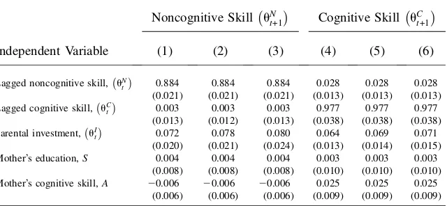
Unanchored Technology Equations:aMeasurement Error is Classical, Absence of Omitted Inputs Correlated withutWhite Males, CNLSY/79
Noncognitive Skill uN t+1
Cognitive Skill uC t+1
Independent Variable (1) (2) (3) (4) (5) (6)
Lagged noncognitive skill, uN t
0.884 0.884 0.884 0.028 0.028 0.028
(0.021) (0.021) (0.021) (0.013) (0.013) (0.013) Lagged cognitive skill, uC
t
0.003 0.003 0.003 0.977 0.977 0.977
(0.013) (0.012) (0.013) (0.038) (0.038) (0.038) Parental investment, uI
t
0.072 0.078 0.080 0.064 0.069 0.071
(0.020) (0.021) (0.024) (0.013) (0.014) (0.015)
MotherÕs education,S 0.004 0.004 0.004 0.003 0.003 0.003
(0.008) (0.008) (0.008) (0.010) (0.010) (0.010) MotherÕs cognitive skill,A 20.006 20.006 20.006 0.025 0.025 0.025
(0.006) (0.006) (0.006) (0.009) (0.009) (0.009)
a. Letu#t¼ uN t;uCt;uIt
denote the noncognitive, cognitive and investment dynamic factors, respectively. LetSdenote mother’s education andAdenote mother’s cognitive ability. The technology equations are:
uk
t+1¼gk1uNt +gk2uCt +g3kuIt+ck1S+ck2A+hkt:
In this table we show the estimated parameter values and standard errors (in parentheses) of
gk
1;gk2;gk3;c
k
1;andc
k
2in Columns 1–6. In Columns 1 and 4, the parental investment factor is normalized
on the log-family income equation. In Columns 2 and 5, the parental investment factor is normalized on trips to the museum. In Columns 3 and 6, we normalize the parental investment factor on trips to the theater.
23. As discussed in Linver, Brooks-Gunn, and Cabrera (2004), some of these items are not useful because they do not vary much among families (that is, more than 90 percent to 95 percent of all families make the same response).
specific behaviors that children aged 4 and older may have exhibited in the previous three months. Three response categories are used in the questionnaire: often true, sometimes true, and not true. In our empirical analysis we use the following sub-scores of the behavioral problems index: (1) antisocial, (2) anxious/depressed, (3) headstrong, (4) hyperactive, (5) peer problems. We standardize these variables so that among other characteristics, a child who scores low on the antisocial subscore is a child who often cheats or tells lies, is cruel or mean to others, and does not feel sorry for misbehaving. A child who displays a low score on the anxious/depressed mea-surement is a child who experiences sudden changes in mood, feels no one loves him/her, is fearful, or feels worthless or inferior. A child with low scores on the headstrong measurement is tense, nervous, argues too much, and is disobedient at home. Children will score low on the hyperactivity subscale if they have difficulty concentrating, act without thinking, and are restless or overly active. Finally, a child will be assigned a low score on the peer problem subscore if they have problems get-ting along with others, are not liked by other children, and are not involved with others.
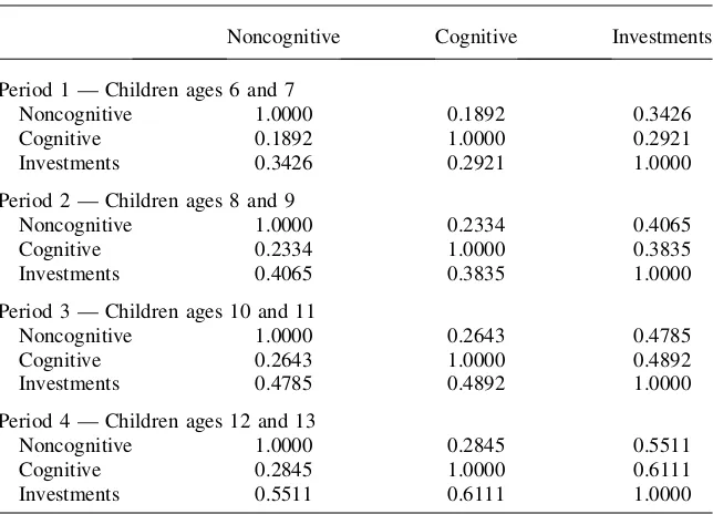
For measurements of cognitive skills we use the Peabody Individual Achievement Test (PIAT), which is a wide-ranging measure of academic achievement of children age five and over. It is commonly used in research on child development. Todd and Wolpin (2005) use the raw PIAT test score as their measure of cognitive outcomes. Table 3
Contemporaneous Correlation Matrices: Measurement Error is Classical, Absence of Omitted Inputs Correlated withut, White Males, CNLSY/79
Noncognitive Cognitive Investments
Period 1 — Children ages 6 and 7
Noncognitive 1.0000 0.1892 0.3426
Cognitive 0.1892 1.0000 0.2921
Investments 0.3426 0.2921 1.0000
Period 2 — Children ages 8 and 9
Noncognitive 1.0000 0.2334 0.4065
Cognitive 0.2334 1.0000 0.3835
Investments 0.4065 0.3835 1.0000
Period 3 — Children ages 10 and 11
Noncognitive 1.0000 0.2643 0.4785
Cognitive 0.2643 1.0000 0.4892
Investments 0.4785 0.4892 1.0000
Period 4 — Children ages 12 and 13
Noncognitive 1.0000 0.2845 0.5511
Cognitive 0.2845 1.0000 0.6111
The CNLSY/79 includes two subtests from the full PIAT battery: PIAT Mathematics and PIAT Reading Recognition.25The PIAT Mathematics test measures a child’s at-tainment in mathematics as taught in mainstream education. It consists of 84 multi-ple-choice items of increasing difficulty. It begins with basic skills such as recognizing numerals and progresses to measuring advanced concepts in geometry and trigonometry. The PIAT Reading Recognition subtest measures word recognition and pronunciation ability. Children read a word silently, then say it aloud. The test contains 84 items, each with four options, which increase in difficulty from preschool to high school levels. Skills assessed include the ability to match letters, name names, and read single words aloud.
Our dynamic factor models allow us to exploit the wealth of measures available in these data. They enable us to solve several problems. First, there are many proxies for parental investments in children’s cognitive and noncognitive development. Even if all parents provided responses to all of the measures of family input, we would still face the problem of selecting which variables to use and how to find enough instru-ments for so many endogenous variables. Applying the dynamic factor model, we let the data tell us the best combination of family input measures to use in predicting the levels and growth in the test scores instead of relying on an arbitrary index. Measured inputs that are not very informative on family investment decisions will have Table 4
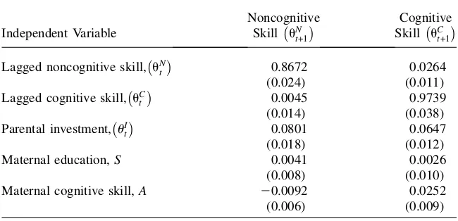
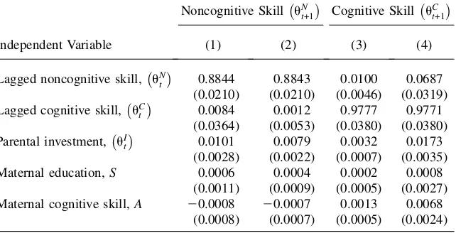
Unanchored Technology Equations:aMeasurement Error is Nonclassical, Absence of Omitted Inputs Correlated withut, White Males, CNLSY/79
Independent Variable
Noncognitive Skill uN
t+1
Cognitive Skill uC
t+1
Lagged noncognitive skill, uN t
0.8672 0.0264
(0.024) (0.011)
Lagged cognitive skill, uC t
0.0045 0.9739
(0.014) (0.038)
Parental investment, uIt
0.0801 0.0647
(0.018) (0.012)
Maternal education,S 0.0041 0.0026
(0.008) (0.010)
Maternal cognitive skill,A 20.0092 0.0252
(0.006) (0.009)
a. Letu#t¼ uN t;u
C t;u
I t
denote the noncognitive, cognitive and investment dynamic factors, respectively. LetSdenote mother’s education andAdenote mother’s cognitive ability. The technology equations are:
uk t+1¼g
k
1u
N t +g
k
2u
C t +g
k
3u
I t+c
k
1S+c
k
2A+h
k t:
In this table we show the estimated parameter values and standard errors (in parenthesis) ofgk
1;gk2;gk3;c
k
1;
andck
2for noncognitive (k¼N) and cognitive (k¼C) skills. Investment is normalized in family income.
estimated factor loadings that are close to zero. Covariance restrictions in our model substitute for the missing instruments to secure identification.
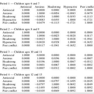
Second, our models have the additional advantage that they help us solve the prob-lem of missing data. It often happens that mothers do not provide responses to all items of the HOME-SF score. Similarly, some children may take the PIAT Reading Recognition exam, but not the PIAT Mathematics test. Another missing data problem that arises is that the mothers may provide information about whether the child has peer problems or not, but may refuse to issue statements regarding the child’s hyper-activity level. For such cases, some researchers drop the observations for the parents who do not respond to certain items, or do not analyze the items that are not responded to by many parents, even though these items may be very informative. With our setup, we do not need to drop the parents or entire items in our analysis. Assuming that the data are missing randomly, we integrate out the missing items Table 5
Contemporaneous Correlation Matrices in Measurement Error: Measurements for Noncognitive Skills, White Males, CNLSY/79
Period 1 — Children ages 6 and 7
Antisocial Anxious Headstrong Hyperactive Peer conflict
Antisocial 1.0000 0.0000 0.0000 0.0000 0.0000
Anxious 0.0000 1.0000 20.0054 20.0083 0.0479
Headstrong 0.0000 20.0054 1.0000 0.0193 20.1113
Hyperactive 0.0000 20.0083 0.0193 1.0000 20.1721
Peer conflict 0.0000 0.0479 20.1113 20.1721 1.0000
Period 2 — Children ages 8 and 9
Antisocial 1.0000 0.0000 0.0000 0.0000 0.0000
Anxious 0.0000 1.0000 20.0023 20.0020 0.0117
Headstrong 0.0000 20.0023 1.0000 0.0328 20.1941
Hyperactive 0.0000 20.0020 0.0328 1.0000 20.1652
Peer conflict 0.0000 0.0117 20.1941 20.1652 1.0000
Period 3 — Children ages 10 and 11
Antisocial 1.0000 0.0000 0.0000 0.0000 0.0000
Anxious 0.0000 1.0000 0.0196 0.0001 20.0007
Headstrong 0.0000 0.0196 1.0000 0.0067 20.0312
Hyperactive 0.0000 0.0001 0.0067 1.0000 20.0002
Peer conflict 0.0000 20.0007 20.0312 20.0002 1.0000
Period 4 — Children ages 12 and 13
Antisocial 1.0000 0.0000 0.0000 0.0000 0.0000
Anxious 0.0000 1.0000 20.0797 20.1495 20.0105
Headstrong 0.0000 20.0797 1.0000 0.0692 0.0049
Hyperactive 0.0000 20.1495 0.0692 1.0000 0.0092
Table 6
Contemporaneous Correlation Matrices in Measurement Error: Measurements for Parental Investments, White Males, CNLSY/79
Income Books Musical Newspaper Lessons Museum Theater
Period 1 — Children ages 6 and 7
Family income 1.0000 0.0000 0.0000 0.0000 0.0000 0.0000 0.0000
Number of books 0.0000 1.0000 20.0044 0.0050 20.0029 20.0269 20.0678
Musical instruments 0.0000 20.0044 1.0000 20.0047 0.0027 0.0257 0.0647
Newspaper subscriptions 0.0000 0.0050 20.0047 1.0000 20.0031 20.0290 20.0731
Number of special lessons 0.0000 20.0029 0.0027 20.0031 1.0000 0.0168 0.0423
Trips to museum 0.0000 20.0269 0.0257 20.0290 0.0168 1.0000 0.3960
Trips to theater 0.0000 20.0678 0.0647 20.0731 0.0423 0.3960 1.0000
Period 2 — Children ages 8 and 9
Family income 1.0000 0.0000 0.0000 0.0000 0.0000 0.0000 0.0000
Number of books 0.0000 1.0000 20.0008 0.0052 0.0018 20.0160 20.0484
Musical instruments 0.0000 20.0008 1.0000 20.0019 20.0006 0.0058 0.0175
Newspaper subscriptions 0.0000 0.0052 20.0019 1.0000 0.0039 20.0355 20.1076
Number of special lessons 0.0000 0.0018 20.0006 0.0039 1.0000 20.0121 20.0366
Trips to museum 0.0000 20.0160 0.0058 20.0355 20.0121 1.0000 0.3291
Trips to theater 0.0000 20.0484 0.0175 20.1076 20.0366 0.3291 1.0000
Period 3 — Children ages 10 and 11
Family income 1.0000 0.0000 0.0000 0.0000 0.0000 0.0000 0.0000
Number of books 0.0000 1.0000 20.0001 20.0001 20.0001 0.0052 0.0007
Musical instruments 0.0000 20.0001 1.0000 0.0002 0.0003 20.0137 20.0017
Newspaper subscriptions 0.0000 20.0001 0.0002 1.0000 0.0002 20.0083 20.0010
Number of special lessons 0.0000 20.0001 0.0003 0.0002 1.0000 20.0130 20.0016
Trips to museum 0.0000 0.0052 20.0137 20.0083 20.0130 1.0000 0.0693
Trips to theater 0.0000 0.0007 20.0017 20.0010 20.0016 0.0693 1.0000
Period 4 — Children ages 12 and 13
Family income 1.0000 0.0000 0.0000 0.0000 0.0000 0.0000 0.0000
Number of books 0.0000 1.0000 0.0003 20.0007 0.0000 0.0017 0.0158
Musical instruments 0.0000 0.0003 1.0000 20.0006 0.0000 0.0016 0.0151
Newspaper subscriptions 0.0000 20.0007 20.0006 1.0000 0.0000 20.0034 20.0313
Number of special lessons 0.0000 0.0000 0.0000 0.0000 1.0000 0.0001 0.0010
Trips to museum 0.0000 0.0017 0.0016 20.0034 0.0001 1.0000 0.0803
Trips to theater 0.0000 0.0158 0.0151 20.0313 0.0010 0.0803 1.0000
The
Journal
of
Human
from the sample likelihood. Appendix 2 presents our sample likelihood. We now pre-sent and discuss our empirical results using the CNLSY data.
A. Empirical Results
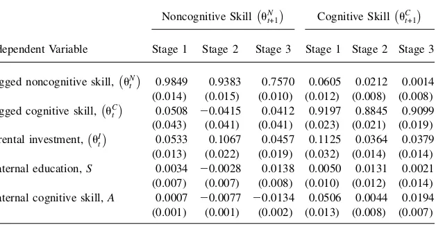
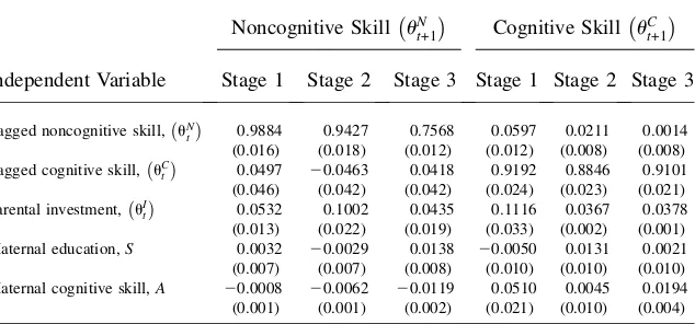
We first present our estimates of an age-invariant version of the technology where we assume no critical and sensitive periods. We report estimates of a model with critical and sensitive periods in Subsection 5 below.
1. Estimates of Time-Invariant Technology Parameters
Using the CNLSY data, we estimate the simplest version of the model that imposes the restriction that the coefficients on the technology equations do not vary over peri-ods of the child’s life cycle, there are no omitted inputs correlated withut, and the
measurement error is classical. In Table 2 we report results in the scale of standard-ized test scores. We normalize the scale of the investment factoruI
ton different
meas-ures. Columns 1 and 4 show the estimated noncognitive and cognitive skill technologies, respectively, when we normalize the investment factor on family come. Columns 2 and 5 show the estimated parameters when we normalize the in-vestment factor on ‘‘trips to the museum.’’ Finally, in Columns 3 and 6 we show the results when we normalize the factor loading in ‘‘trips to the theater.’’ The esti-mated technology is robust to different normalization assumptions.26
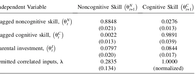
Table 7
Unanchored Technology Equations:aMeasurement Error is Classical, Allows for Omitted InputlCorrelated withut, White Males, CNLSY/79
Independent Variable Noncognitive Skill uN
t+1
Cognitive Skill uC t+1
Lagged noncognitive skill, uN t
0.8848 0.0276
(0.021) (0.013)
Lagged cognitive skill, uC t
0.0022 0.9891
(0.013) (0.039)
Parental investment, uI t
0.0797 0.0844
(0.020) (0.017)
Omitted correlated inputs,l 0.2835 1.0000
(0.134) (normalized)
a. Letu#t¼ uN t;uCt;uIt
denote the noncognitive, cognitive and investment dynamic factors, respectively. Letldenote omitted inputs that are potentially correlated withut. The technology equations are:
uk
t+1¼gk1uNt +gk2uCt +gk3uIt+gk4l+nkt:
In this table we show the estimated parameter values and standard errors (in parentheses) of
gk
1;gk2;gk3andgk4:Note that for identification purposes we normalizegC4 ¼1:Investment is normalized
on family income.
Table 2 shows the estimated parameter values and their standard errors. From this table, we see that: (1) both cognitive and noncognitive skills show strong persistence over time; (2) noncognitive skills in one period affect the accumulation of next pe-riod cognitive skills, but cognitive skills in one pepe-riod do not affect the accumulation of next period noncognitive skills; (3) the estimated parental investment factor affects noncognitive skills slightly more strongly than cognitive skills, but the differ-ences are not statistically significant; (4) the mother’s ability affects the child’s cog-nitive ability but not noncogcog-nitive ability; (5) the mother’s education plays no role in affecting the evolution of ability after controlling for parental investments, and moth-er’s ability. We contrast the OLS estimates of this model (presented in Table 16) with our measurement-error corrected versions in Subsection 6 below.
The dynamic factors are statistically dependent. Table 3 shows the evolution of the correlation patterns across the dynamic factors. The correlation between cognitive and noncognitive skills is 0.18 at ages six and seven, and grows to around 0.28 at ages 12 and 13. There is a strong contemporaneous correlation among noncognitive skill and the home investment. The correlation starts off at 0.40 at ages six and seven and grows to 0.55 by ages 12 and 13. The same pattern is true for the correlation between cognitive skills and home investments. The correlation between these two variables goes from 0.38 at ages six and seven to 0.61 at ages 12 and 13.
2. Allowing for Nonclassical Measurement Error
We check the robustness of our findings by relaxing the assumption that the error terms in the measurement equations are classical. We allow the measurement errors (except for the first measurement) to be freely correlated and estimate their depen-dence. Table 4 shows the estimated technologies for noncognitive and cognitive skills estimated under these more general conditions.27The main conclusions based on Table 2 are robust to the assumption that measurement error is classical.28In Ta-ble 5 we show the estimated contemporaneous correlation across the measurement errors in our measures of noncognitive skills. Most of the correlations across the er-ror terms are low. In fact, no correlation in any period exceeds, in absolute value, 0.2, and most are well below it.
Table 6 reports the contemporaneous correlation of the error terms in the measure-ment equations for investmeasure-ment. We assume that the error term in family income is independent of the remaining error terms. Virtually all correlations are well below 0.04 in absolute value. The only exceptions are the correlations between ‘‘trips to the museum’’ and ‘‘trips to the theater’’ in Periods 1 and 2. In sum, these findings suggest that the assumption that the measurement error is classical is not at odds with the data we analyze, and allowing for correlation in errors does not change the main conclusions obtained from the simpler technology assuming classical measurement error.
27. We use family income to normalize investment.