Directory UMM :Data Elmu:jurnal:E:Energy Economics:Vol22.Issue2.2000:

(1)

A multivariate cointegration analysis of the

role of energy in the US macroeconomy

David I. Stern

U

Centre for Resource and En¨ironmental Studies, Australian National Uni¨ersity, Canberra, ACT 0200, Australia

Abstract

This paper extends my previous analysis of the causal relationship of GDP and energy use in the USA in the post-war period. A majority of the relevant variables are integrated justifying a cointegration analysis. The results show that cointegration does occur and that energy input cannot be excluded from the cointegration space. The results are plausible in terms of macroeconomic dynamics. The results are similar to my previous Granger causality

Ž .

JEL classification:Q41

Keywords:Energy; GDP; Cointegration; United States

1. Introduction

Ž .

Stern 1993 addressed the debate among economists and energy analysts regard-Ž

ing the role of energy in the US macroeconomy. Several analysts Kraft and Kraft, 1978; Akarca and Long, 1980; Yu and Hwang, 1984; Abosedra and Baghestani,

. Ž . Ž .

1991 have used Granger 1969 or Sims 1972 tests to test whether energy use causes economic growth or whether energy use is determined by the level of output. The results are generally inconclusive. Where significant results were

U

Tel.:q61-2-6249-0664; fax:q61-2-6249-0757.

Ž .

E-mail address:dstern@cres.anu.edu.au D.I. Stern

(2)

( ) D.I. SternrEnergy Economics 22 2000 267]283 268

obtained they indicate that causality runs from output to energy use. Erol and Yu

Ž1987 found some indications of a causal relationship between energy and output.

in a number of industrialised countries with the most significant relationship being for Japanese data between 1950 and 1982. However, when the sample was

re-stricted to 1950]1973 the relationship was no longer significant. Yu and Choi

Ž1985 also found a causal relationship running from energy to GDP in the.

Philippines economy, and causality from GDP to energy in the economy of South Korea. In the latter economy, causality from energy to GDP is significant only at

Ž .

the 10% level. Ammah-Tagoe 1990 found causality from GDP to energy use in Ghana.

Ž .

My previous study Stern, 1993 tested for Granger causality in a multivariate

Ž .

setting using a vector autoregression VAR model of GDP, energy use, capital, and labour inputs. I also used a quality-adjusted index of energy input in place of gross energy use. The multivariate methodology is important because changes in energy use are frequently countered by the substitution of other factors of production, resulting in an insignificant overall impact on output. Weighting energy use for changes in the composition of energy input is important because a large part of the growth effects of energy are due to substitution of higher quality energy

Ž

sources such as electricity for lower quality energy sources such as coal Jorgenson, .

1984; Hall et al., 1986; Kaufmann, 1994 . When both these innovations are employed, energy is found to Granger cause GDP. These results are supported by

Ž . Ž .

Hamilton 1983 and Burbridge and Harrison 1984 , who found that changes in oil prices Granger-cause changes in GNP and unemployment in VAR models whereas

Ž .

oil prices are exogenous to the system. More recently, Moroney 1992 presented a

Ž .

theoretical and empirical analysis that counters the argument of Perry 1977 ,

Ž . Ž .

Solow 1978 , Denison 1979, 1985 , and others, that because energy costs are only a small proportion of GDP, energy use is unlikely to be a very important factor in

Ž .

changing the rate of economic growth. Moroney 1992 uses a labour-intensive form of a production function with capital embodied technological change to investigate the effects of changes in capital and energy used per unit of labour on labour productivity. The estimates of the output elasticities are similar for both the latter variables. Furthermore, a breakdown of the sources of growth shows that in

the period 1950]1973 changes in energy used per unit of labour contributed an

annual average 1.17 percentage points to economic growth, while from 1974 to 1984 declines in energy use reduced growth by an annual average of 0.5 percentage points.

Ž .

(3)

energy efficiency, shifts in the composition of the energy input, and structural change in the economy, mean that energy and output will drift apart. Similar

comments apply to the bivariate energy]employment relationship. Furthermore,

the insensitivity of the test may be compounded by using total energy in the economy as a whole but measuring output as industrial output alone.

Ž .

Masih and Masih 1996 find cointegration between energy and GDP in India, Pakistan, and Indonesia, but no cointegration in Malaysia, Singapore, or the Philippines. Granger causality runs from energy to GDP in India but in the opposite direction in the other two countries.

Ž . Ž .

Ohanian 1988 and Toda and Phillips 1993 showed that the distribution of the test statistic for block exogeneity in a VAR with non-stationary variables is not the

standard x2 distribution. This means that the significance levels reported in

previous studies of the Granger-causality relationship between energy and GDP may be incorrect, as both variables are generally integrated series. If there is no cointegration between the variables then the causality test should be carried out on

a VAR in differenced data, while if there is cointegration, standardx2_{distributions}

apply when the cointegrating restrictions are imposed. Thus, testing for cointegra-tion is a necessary prerequisite to causality testing.

It seems that if a multivariate approach helps in uncovering the Granger causality relations between energy and GDP a multivariate approach should be used to investigate the cointegration relations among the variables. In this paper, I investigate the time series properties of GDP, quality weighted energy, labour, and capital series, estimate some simple static single equation production functions, and estimate three versions of a dynamic cointegration model using the Johansen methodology. The methods are outlined in Section 2 of the paper, which is followed by the results and finally some conclusions.

2. Methodology

2.1. General

The basic model is a four equation VAR on annual data for US GDP, energy input, capital input, and labour input, between 1948 and 1994. The general form of the VAR is:

where GDP is gross domestic product, K is capital input, L is labour input, and E

ŽŽ . .

is energy input.r is the number of lags,G is a 4?r q2 =4 matrix of regression

(4)

capture the effects of exogenous technical change. The optimum lag length r was

chosen using the Hannan]Quinn Information Criterion. The maximum lag length

considered is four. Energy input is measured by a quality-adjusted index of final Ž energy use. This quality-adjusted index is created using Divisia aggregation see

. Appendix A for details .

2.2. Tests for integration

Ž .

The variables in Eq. 2 may be integrated. I test this hypothesis using four ‘unit

Ž .

root tests’. The Dickey]Fuller Dickey and Fuller, 1979, 1981 and Phillips]Perron

ŽPhillips and Perron, 1988 tests are the same but use different approaches to cope.

with serial correlation in the data. For both tests, the null-hypothesis is that the

series has a stochastic trend. The model for the Dickey]Fuller test is:

p

Ž .

Dytsaqbtqgyty1q

_Ý

d Di ytyiq«t 3

is1

where y is the variable under investigation and «t is a random error term. The

Ž .

number of lags pis chosen using the Akaike Information Criterion Akaike, 1973 .

The maximum lag length considered is four. The lagged variables provide a

correction for possible serial correlation. The null hypothesis is given by gs0.

Ž .

This is tested using the t-statistic tt in Table 1 which has a non-standard

distribution. The alternative hypothesis is that the process is stationary around the deterministic trend. A further battery of tests looks at other alternatives including

Ž .

levels stationarity. In the model above Model 1 in Table 1 the test t_{a t} is a t-test

on the parameter a given that gs0, and t_{b t} tests bs0 given that gs0. The

statistics f2 andf3 areF-type statistics.f2evaluates the joint restriction asbs

gs0 whilef₃evaluates the joint restriction bsgs0. Model 2 in Table 1 is the

Ž .

same as Eq. 3 but without the deterministic time trend. If the data do not contain a deterministic trend then this model should provide a more powerful test of the

Table 1

a Dickey]Fuller statistics

Variables Lags Model 1 Model 2 Model 3Model 3

t

(5)

unit root hypothesis.tm,ta m, and f1 correspond to the statistics tt,ta t, and f3 in Ž .

Model 1. Model 3 excludes both the constant and time trend from Eq. 3 . The only relevant test statistic is t, a t-test for gs0. I do these tests in the order suggested

Ž .

by Dolado et al. 1990 .

The Phillips]Perron test uses the same models as the Dickey]Fuller tests, but

Ž .

uses a non-parametric correction, due to Newey and West 1987 , to cope with potential serial correlation. I chose the lag truncation for this non-parametric correction using an automated bandwidth estimator employing the Bartlett kernel ŽAndrews, 1991 . The test statistics for both the Dickey. ]Fuller and Phillips]Perron

Ž .

tests have the same distributions. Critical levels are reproduced in Hamilton 1994

Ž .

and Enders 1995 .

Ž .

The model used in the Schmidt]Phillips test Schmidt and Phillips, 1992 is given

by:

where T is the number of observations, and «_t is a random error term. First the

Ž . Ž .

‘residual’ St is computed using Eq. 5 and then the regression in Eq. 4 is

estimated. The test statistic is again a t-test on g. The null is again the presence of a stochastic trend, while the alternative is trend stationarity. Critical values for the

Ž .

test statistic are presented in Schmidt and Phillips 1992 . I use the same correction for serial correlation as for the Phillips]Perron test.

Ž . Ž .

The Kwiatowski et al. 1992 test KPSS differs from the other three tests in that the null hypothesis postulates that the series is stationary and the alternative hypothesis is the presence of a stochastic trend. A second version has a null of trend stationarity. The test statistic is a Lagrange Multiplier statistic, which is calculated as the square of the sum of residuals divided by the estimated error variance from a regression of the variable in question on either a constant or a

constant and a trend. I again use the AndrewsrNewey-West procedure to correct

for serial correlation.

2.3. Cointegration analysis

On condition that at least some of the variables are integrated, the VAR model

Ž . Ž .1 , 2 can be estimated subject to cointegrating restrictions. Maximum likelihood

Ž

estimation is carried out using the Johansen procedure Johansen, 1988; Johansen .

and Juselius, 1990 . Practical and theoretical background is given by Hamilton Ž1994 , Enders 1995 and Hansen and Juselius 1995 .. Ž . Ž .

Ž .

(6)

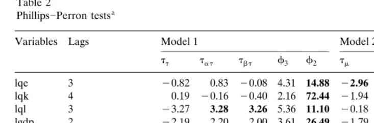
Table 2

a Phillips]Perron tests

Variables Lags Model 1 Model 2 Model 3

t

Figures in bold indicate that the statistic is significant at the 5% level.

These are the two most important hypotheses to be tested in the cointegration analysis.

Some initial specification testing is also carried out with single equation

Cobb]Douglas production functions estimated using ordinary least squares. These

are the Engle]Granger cointegrating regressions corresponding to the vector

autoregression model in logarithms.

3. Results

3.1. Tests for integration

Ž .

The Dickey]Fuller test suite Table 1 provides mixed evidence on the order of

integration. Looking at the statistics for model 1 for energy, capital, and GDP, we Ž .

can accept the hypothesis that the series contain a unit root tt and that there is

Ž . Ž .

neither a constant ta,f3 nor a deterministic time trend tb in the process. But

the test for a drift term is not very powerful in the presence of the deterministic

trend in the regression as shown by the fact that the joint restrictionasbsgs0

Ž .

is rejected. The Dolado et al. 1990 algorithm suggests estimation of model 2,

Table 3

a Schmidt}Phillips tests

Variable Lags t Zt

lqe 1 y0.94536 y0.99413

lqk 4 y0.65845 y0.95208

lql 2 y3.25773 y3.53376

lgdp 1 y1.78818 y1.92883

a

(7)

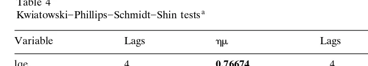
Table 4

a Kwiatowski]Phillips]Schmidt]Shin tests

Variable Lags hm Lags ht

lqe 4 0.76674 4 0.27111

lqk 4 0.85094 4 0.25229

lqh 4 0.86448 4 0.05521

lgdp 4 0.83443 4 0.25361

a

The null is stationarity. hm is the test statistic against levels stationarity,ht is the test statistic against trend stationarity. Figures in bold indicate that the statistic is significant at the 5% level.

which excludes the deterministic time trend a priori. The t_m test suggests that the

Ž

energy and capital series are levels stationary with a significant constant as shown .

by ta m and f1 . The 5% significance level for tm is ]2.89. This result is suspect

because both these series are strongly trending. For GDPtm indicates that the data

have a unit root while f₁ rejects restriction of the constant to zero. This series is

more clearly a random walk with drift. For labour, the tests for model 1 reject the unit root hypothesis and suggest the inclusion of a linear time trend. According to this test labour is trend stationary.

Ž .

The Phillips]Perron test Table 2 indicates that capital, labour, and GDP are

integrated. The tm statistic is significant at the 5% level for the energy input

variable, which would indicate that the series is level stationary. Given that the variable has a strong trend up until 1973 this result is anomalous.

Ž .

The Schmidt]Phillips test results Table 3 indicate the acceptance of the unit

root hypothesis for energy, capital, and GDP at the 5% significance level, but at the 1% significance level all variables, including labour, are found to be integrated.

Ž .

The KPSS test Table 4 shows that all the variables with the exception of labour input are integrated with drift when compared to a trend stationary specification. Labour input is trend stationary.

In conclusion, the univariate tests seem to show that energy, capital, and GDP are integrated variables while labour is more likely to be trend stationary.

3.2. Single equation specification and cointegration tests

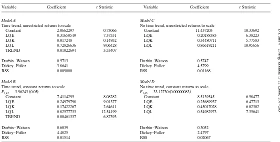
Table 5 presents estimates of four different Cobb]Douglas aggregate production

Ž .

functions. These are static cointegrating or spurious regressions, which corre-spond to the long-run relation in the vector autoregression model in logarithms

presented below. The Cobb]Douglas production function unrealistically imposes a

unitary elasticity of substitution between all factors of production. This restriction is justifiable because: more flexible functional forms, such as the translog, are difficult to estimate in the VAR context with the available length of time series; and accurate single equation static estimates of flexible functional forms are also very difficult to obtain due to multicollinearity. Model A is a production function

(8)

()

Variable Coefficient tStatistic Variable Coefficient tStatistic

Model A Model C

Time trend, unrestricted returns to scale No time trend, unrestricted returns to scale

Constant y2.0662297 y0.73066 Constant y11.437203 y10.33692

LQE 0.31650549 7.37551 LQE 0.20188383 6.38223

LQK y0.017248 y0.14952 LQK 0.34480711 5.77583

LQL 0.72826636 9.06428 LQL 0.86619211 10.95656

TREND 0.01022694 3.53407

Durbin]Watson 0.5713 Durbin]Watson 0.5747

Dickey]Fuller y3.8641 Dickey]Fuller y4.5799

RSS 0.009000 RSS 0.01168

Model B Model D

Time trend, constant returns to scale No time trend, constant returns to scale

Ž . Ž .

F1,42s3.96243 0.05 F1,43s33.12730 0.00000083

Constant y7.4114295 y8.08282 Constant y8.5139545 y6.58477

LQE 0.24979798 9.01377 LQE 0.25689937 6.47713

LQK 0.17422267 2.64611 LQK 0.45017028 6.02302

LQL 0.82577733 12.54199 LQL 0.54982973 7.35641

TREND 0.00461337 6.87393

Durbin]Watson 0.6039 Durbin]Watson 0.3052

Dickey]Fuller y4.4825 Dickey]Fuller y2.4797

RSS 0.01514 RSS 0.02067

a

(9)

Ž .

indicates that there is cointegration Engle and Granger, 1987 , the coefficient on

capital input is insignificant and has the wrong sign. The Dickey]Fuller

cointegra-tion statistic is only just significant at the 10% level. Model B imposes a restriccointegra-tion so that GDP exhibits constant returns to scale in capital and labour. This restric-tion can just be accepted at the 5% level. Now all the coefficients are significant.

The Dickey]Fuller statistic shows that we can reject the non-cointegration

hy-pothesis at a higher level of significance. The estimated rate of technical change is lower than before. As the coefficient of energy is significant and positive, we find that there are increasing returns in terms of GDP when energy and the two primary inputs are all increased. Some of this effect is absorbed by the time trend in the unrestricted model.

Model C is a Cobb]Douglas function without a time trend and with unrestricted

returns to scale. All the input coefficients have the expected sign and are signifi-cant. There are increasing returns to scale to both capital and labour alone and to all three inputs. There is cointegration. Model D imposes constant returns to primary inputs on Model C. This restriction is, however, easily rejected and the equation no longer cointegrates.

Though the time trend is significant in models A and B, model C has a better fit to the data than model B. Models B and C have the best cointegration properties. These results show that the system can be represented as either one with constant returns in capital and labour and exogenous technical change or as an unrestricted increasing returns specification with no exogenous technical change. The latter

Ž .

model can be estimated using the CATS package Hansen and Juselius, 1995 while

the constant returns to scale restriction cannot be implemented in that package.1

Also the increasing returns approach is more compatible with the idea of en-dogenous technical change. However, models with time trends are also estimated in the multivariate analysis.

3.3. Multi¨ariate cointegration analysis

The optimal lag length is selected using the information criteria in Table 6. These statistics refer to a model with a constant restricted to the cointegration

space and no time trends. According to the Hannan]Quinn criterion the optimal

lag length is two lags. The Schwartz criterion favours only one lag. I choose two lags because this allows for short-run dynamics in the vector error correction model and the residual properties of the two lag models are also very adequate compared to the other models. This was assessed using the array of serial

correlation, ARCH and normality statistics provided by the CATS program.2 _Table

1

The constant returns restriction could be implemented by estimating a VAR in terms of the variables

Ž . Ž .

ln GDPrL, lnKrL, and lnE. 2

These tests are: Lagrange multiplier tests for first order and fourth order multivariate serial correla-tion, the Ljung]Box multivariate autocorrelation test, a multivariate normality test, and univariate tests

Ž .

(10)

Table 6

Selection of lag length

Number of lags Log likelihood Schwartz Hannan]Quinn

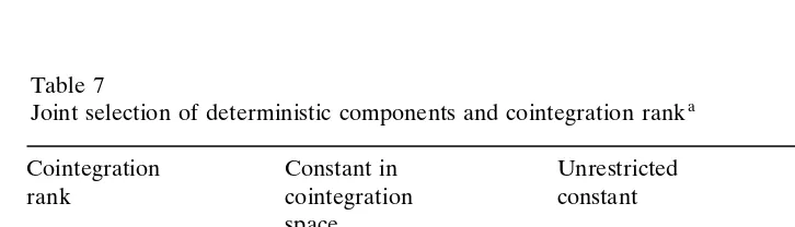
function criterion criterion Joint selection of deterministic components and cointegration rank

Cointegration Constant in Unrestricted Trend in

rank cointegration constant cointegration

The first figure is the Johansen trace cointegration statistic. Figures in parentheses are the 90% critical values of the trace cointegration statistic.

7 reports the Johansen trace cointegration test statistics and 90% critical values for

cointegration ranks of 1, 2, and 3} as there are four equations a rank of 4 would

imply that the model was stationary } and different deterministic specifications.

These results are for two lags. Restriction of the cointegration rank to one is rejected. Any model of rank 2 is acceptable. As a consequence I estimate all three rank 2 models.

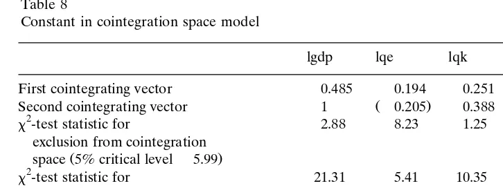
Table 8 presents the results for the model with the constant restricted to the cointegration space which is equivalent to the static Model C described above. On the basis of the values of the parameters the second cointegrating vector is clearly a production function. Because of this I have not tested identifying restrictions of the vectors as this would imply setting at least one of the coefficients in this equation to zero. The exclusion test statistics suggest that the relation could, however, be identified by excluding capital. The most important result from the point of view of this paper is that energy cannot be excluded from this cointegrat-ing relation. Energy is, however, the only variable that can be considered weakly

exogenous. As shown by the t statistics for alpha the second cointegrating vector

(11)

Table 8

Constant in cointegration space model

lgdp lqe lqk lql Constant

First cointegrating vector y0.485 0.194 y0.251 1 y4.489

Ž .

Second cointegrating vector 1 y0.205 y0.388 y0.935 4.273

2

x-test statistic for 2.88 8.23 1.25 8.86 8.93

exclusion from cointegration

Ž .

space 5% critical levels5.99 2

x-test statistic for 21.31 5.41 10.35 15.50 ]

Ž .

weak exogeneity 5% critical levels5.99

Ž

First column of alpha tstats 0.092 0.029 0.004 0.091 ]

. Ž . Ž . Ž . Ž .

in parentheses 4.612 1.094 0.818 4.623

Ž

Second column of alpha t 0.4 0.283 0.086 0.155 ]

. Ž . Ž . Ž . Ž .

stats in parentheses 4.505 2.387 4.157 1.775

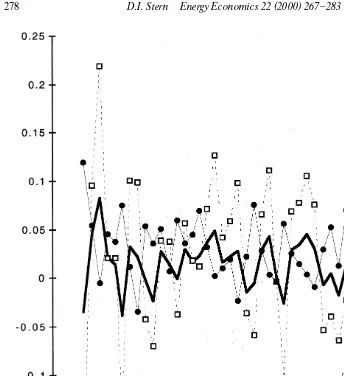
labour equations. I have therefore normalised it on labour. It could possibly be interpreted as a labour supply function. I investigate this hypothesis by plotting in Fig. 1 the percentage changes in the long-run equilibrium values of labour predicted by the two cointegrating relations. Actual labour use closely follows the predicted value from the first cointegrating vector, albeit with a smaller variance.

The predicted value from the production function } the second cointegrating

vector}moves in the opposite direction to actual labour use or rather labour use

responds with a lag to changes in labour demand. From Table 8 we can see that, in the long-run, disequilibrium between labour demand and supply closes at 14%

Ž0.935=0.155 per year. This fits the stylised fact that declines in unemployment.

tend to lag GDP growth. However, labour use tends to accelerate further in response to disequilibrium in the first cointegrating relation. This is a labour

discouragementrencouragement accelerator. In recessions labour use is below

long-run equilibrium but more workers are discouraged from searching. In booms more labour enters the work-force when labour supply is above equilibrium. GDP obviously responds positively to this labour oversupply.

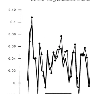
The alpha coefficient that loads the production function relation into the GDP equation is also positive. When GDP is above its long-run equilibrium it tends to accelerate further and vice versa. As can be seen in Fig. 2, GDP is normally below equilibrium during booms and above equilibrium in recessions.

(12)

Fig. 1. Predicted percentage changes in equilibrium values for labor input.

first cointegrating vector loads into the capital equation. So perhaps in this case the first cointegrating relation can be interpreted as a capital accelerator function rather than as a labour demand function. Accordingly I have normalised the vector

on capital. The sign of the relevant alpha coefficient is negative } when there is

over-accumulation of capital there is a regression to equilibrium. Plots of the two

Ž .

(13)

Fig. 2. Predicted percentage changes in equilibrium values for GDP.

Table 10 shows the results that occur when a linear trend is included in the cointegration space. The coefficient signs are the same as in the model with the constant restricted to the cointegration space. The time trend in the production function is 0.9% which is very close to the 1.0% rate estimated in the static model

Ž .

in Table 5 Model A . However, the output elasticity estimates are superior in this dynamic model in that they all have the correct sign but there are actually

Ž .

decreasing returns to capital and labour and roughly constant returns 1.08 to all three factors of production. The negative trend coefficient in the first cointegrating vector indicates that labour supply tends to decline when holding the other inputs constant. This expresses stylised facts such as increased use of capital per worker and the tendency to a shorter working week over time. Again capital can be excluded from the cointegration space but energy is not weakly exogenous. Both cointegrating vectors now have a significant effect on energy use. So, in this model there is more a case of mutual causality between energy and GDP as in Stern

(14)

Table 9

Unrestricted constant model

lgdp lqe lqk lql

First cointegrating vector y0.314 y0.123 1 y0.787

Second cointegrating vector 1 y0.232 y0.206 y1.137

2

x-test statistic for exclusion 3.28 7.55 1.41 7.19

from cointegration space

Ž5% critical levels5.99.

2

x-test statistic for weak exogeneity 8.10 8.09 7.31 8.12

Ž5% critical levels5.99. Ž

First column of alpha tstats y0.0016 y0.017 y0.012 0.0448

. Ž . Ž . Ž . Ž .

in parentheses 0.091 y0.611 y2.321 2.167

Ž

Second column of alpha tstats 0.797 0.701 0.120 0.594

. Ž . Ž . Ž . Ž .

in parentheses 4.666 3.160 3.030 3.589

the more restricted models. The patterns of the cointegrating relations are some-what different than in the previous examples but still the effects on each of the

variables of the two CVs move in opposite directions } cyclical and

countercycli-cal.

4. Conclusions

Both the single equation static cointegration analysis and the multivariate dynamic cointegration analysis show that energy is significant in explaining GDP. They also show that there is cointegration in a relationship including GDP, capital, labour, and energy. This result contradicts the bivariate analysis of Yu and Jin

Ž1992 for the United States. Masih and Masih 1996 found cointegration between. Ž .

energy and GDP in three of the six Asian countries that they investigated, but only

Table 10

Trend in cointegration space model

lgdp lqe lqk lql Trend

First cointegrating vector y1.174 0.354 y0.191 1 0.014

Second cointegrating vector 1 y0.237 y0.157 y0.689 y0.009

2

x-test statistic for exclusion 13.24 18.08 1.62 17.92 11.48

from cointegration space

Ž5% critical levels5.99.

2

x-test statistic for weak 11.80 16.13 8.18 16.27 ]

Ž .

exogeneity 5% critical levels5.99

Ž

First column of alpha tstats 0.046 0.053 y0.005 0.087 ]

. Ž . Ž . Ž . Ž .

in parentheses 2.005 2.150 y0.974 4.239

Ž

Second column of alpha tstats 1.155 1.624 0.229 0.801 ]

. Ž . Ž . Ž . Ž .

(15)

in India did they find cointegration together with causality running from energy to GDP. This study differs from those two by including capital and labour variables and using a quality weighted index of energy input. The multivariate analysis shows that energy Granger causes GDP either unidirectionally as indicated by the first of the three models investigated or possibly through a mutually causative relationship as indicated by the latter two models examined. These results support the

conclu-Ž .

sions of Stern 1993 regarding Granger causality between energy and GDP. The results presented in this paper, strengthen my previous conclusions that energy is a limiting factor in economic growth. Shocks to energy supply will tend to reduce output.

Acknowledgements

I thank Robert Kaufmann and an anonymous referee for many useful comments.

Appendix A. Data sources and construction

Ž .

Detailed sources of data are described in Stern 1993 . That database was

Ž .

updated to 1994 from 1990 and all prices based on 1987 constant dollars. The following additional changes or improvements were made:

Labour is measured in terms of hours worked by full-time and part-time employees in domestic industries.

Capital is measured as the aggregate value of the non-residential private and government net capital stock in constant 1987 dollars. The capital series were updated from 1993 to 1994 using data on investment in 1994.

Ž .

Energy is measured as a Divisia index of the energy content BTU of the final use of coal, natural gas, petroleum, electric power, and biofuels. These categories reflect changes that the Energy Information Administration has made in the way it reports energy data since 1990. The major change is expanded reporting of non-utility production of electricity and renewable energy sources. Final use of the fossil fuels is calculated as the primary inputs minus the amounts used in genera-tion by electric utilities. Use of fossil fuels by non-utility electricity producers are considered as final use. This is so as to avoid a break in the data in 1989 when non-utility coverage is expanded. All use of biofuels by non-utilities is considered

as final use } consumption by utilities is subtracted. All geothermal, solar, and

wind power is included in terms of electricity produced regardless of whether it is produced by utilities or non-utilities.

Fossil fuel prices for the aggregation were improved by using the expenditure Ž

data reported in the Annual Energy Re¨iew US Department of Energy, Energy

.

(16)

References

Abosedra, S., Baghestani, H., 1991. New evidence on the causal relationship between United States energy consumption and gross national product. J. Energy Dev. 14, 285]292.

Akaike, H., 1973. Information theory and an extension of the maximum likelihood principal. In: Petrov,

Ž .

B.N., Csaki, F. Eds. , 2nd International Symposium on Information Theory. Akademini Kiado, Budapest, pp. 267]281.

Akarca, A., Long, T., 1980. On the relationship between energy and GNP: a reexamination. J. Energy Dev. 5, 326]331.

Ammah-Tagoe, F.A., 1990. On Woodfuel, Total Energy Consumption and GDP in Ghana: A Study of Trends and Causal Relations, Center for Energy and Environmental Studies. Boston University,

Ž .

Boston, MA mimeo .

Andrews, D.W.K., 1991. Heteroskedasticity and autocorrelation consistent covariance matrix estimation. Econometrica 59, 817]858.

Burbridge, J., Harrison, A., 1984. Testing for the effects of oil prices rises using vector autoregressions. Int. Econ. Rev. 25, 459]484.

Denison, E., 1979. Explanations of declining productivity growth. Surv. Curr. Bus. August, 1]24. Denison, E., 1985. Trends in American Economic Growth, 1929]1982. The Brookings Institution,

Washington, DC.

Dickey, D.A., Fuller, W.A., 1979. Distribution of the estimators for autoregressive time series with a unit root. J. Am. Stat. Ass. 74, 427]431.

Dickey, D.A., Fuller, W.A., 1981. Likelihood ratio statistics for autoregressive processes. Econometrica 49, 1057]1072.

Dolado, J., Jenkinson, T., Sosvilla-Rivero, S., 1990. Cointegration and unit roots. J. Econ. Surv. 4, 249]273.

Enders, W., 1995. Applied Econometric Time Series. John Wiley, New York.

Engle, R.E., Granger, C.W.J., 1987. Cointegration and error-correction: representation, estimation, and testing. Econometrica 55, 251]276.

Erol, U., Yu, E.S.H., 1987. On the causal relationship between energy and income for industrialized countries. J. Energy Dev. 13, 113]122.

Granger, C.W.J., 1969. Investigating causal relations by econometric models and cross-spectral methods. Econometrica 37, 424]438.

Hall, C.A.S., Cleveland, C.J., Kaufmann, R.K., 1986. Energy and Resource Quality: The Ecology of the Economic Process. Wiley Interscience, New York.

Hamilton, J.D., 1983. Oil and the macroeconomy since World War II. J. Pol. Econ. 91, 228]248. Hamilton, J.D., 1994. Time Series Analysis. Princeton University Press, Princeton, NJ.

Hansen, H., Juselius, K., 1995. CATS in RATS: Cointegration Analysis of Time Series. Estima, Evanston, IL.

Johansen, S., 1988. Statistical analysis of cointegration vectors. J. Econ. Dynam. Control 12, 231]254. Johansen, S., Juselius, K., 1990. Maximum likelihood estimation and inference on cointegration with

application to the demand for money. Oxf. Bull. Econ. Stat. 52, 169]209.

Ž .

Jorgenson, D.W., 1984. The role of energy in productivity growth. Energy J. 5 3 , 11]26.

Kaufmann, R.K., 1994. The relation between marginal product and price in US energy markets:

Ž .

implications for climate change policy. Energy Econ. 16 2 , 145]158.

Kraft, J., Kraft, A., 1978. On the relationship between energy and GNP. J. Energy Dev. 3, 401]403. Kwiatowski, D., Phillips, P.C.B., Schmidt, P., Shin, Y., 1992. Testing the null hypothesis of stationarity

against the alternative of a unit root: how sure are we that economic time series have a unit root. J. Econom. 54, 159]178.

Masih, A.M.M., Masih, R., 1996. Energy consumption, real income and temporal causality: results from a multi-country study based on cointegration and error-correction modelling techniques. Energy Econ. 18, 165]183.

(17)

Newey, W.K., West, K.D., 1987. A simple positive semi-definite heteroskedasticity and autocorrelation consistent covariance matrix. Econometrica 55, 1029]1054.

Ohanian, L.E., 1988. The spurious effects of unit roots on vector autoregressions: a Monte Carlo study. J. Econom. 39, 251]266.

Perry, G.L., 1977. Potential output and productivity. Brookings Papers on Economic Activity 1. Phillips, P.C.B., Perron, P., 1988. Testing for a unit root in time series regression. Biometrika 75,

335]346.

Schmidt, P., Phillips, P.C.B., 1992. LM tests for a unit root in the presence of deterministic trends. Oxf. Bull. Econ. Stat. 54, 257]287.

Sims, C.A., 1972. Money, income and causality. Am. Econ. Rev. 62, 540]552. Solow, R.M., 1978. Resources and economic growth. Am. Econ. 22, 5]11.

Stern, D.I., 1993. Energy use and economic growth in the USA, a multivariate approach. Energy Econ. 15, 137]150.

Toda, H.Y., Phillips, P.C.B., 1993. The spurious effect of unit roots on vector autoregressions: an analytical study. J. Econom. 59, 229]255.

US Department of Energy, Energy Information Administration, 1992. Annual Energy Review 1991. Washington, DC: Government Printing Office.

US Department of Energy, Energy Information Administration, 1995. Annual Energy Review 1994. Washington, DC: Government Printing Office.

Yu, E.S.H, Choi, J.-Y., 1985. The causal relationship between energy and GNP: An international comparison. J. Energy Dev. 10, 249]272.

Yu, E.S.H., Hwang, B., 1984. The relationship between energy and GNP: further results. Energy Econ. 6, 186]190.