Application of factorial kriging for mapping soil variation
at field scale
S. Bocchi
a,*, A. Castrignano`
b, F. Fornaro
b, T. Maggiore
aaDipartimento di Produzione Vegetale sezione Agronomia,
6ia Celoria2,20133Milan,Italy
bIstituto Sperimentale Agronomico,
6ia C.Ulpiani5,70125Bari,Italy
Received 3 November 1999; received in revised form 23 March 2000; accepted 4 May 2000
Abstract
Use of precision farming technologies requires better understanding of soil variability in physical, hydraulic and chemical properties. Some of that variation is natural, some is the result of the management history of the field. So, to match agricultural inputs and practices to site-specific conditions, the factorial kriging algorithm (FKA) was used to analyze spatial variability in some soil physical, hydraulic and chemical properties (sand and silt concentrations, water contents corresponding to potentials of −10, −50, −100, −200, −1000 and −1500 kPa and organic C concentration), measured at two depths within a single field in north Italy. A linear model of coregionalization, including, (1) a nugget effect; (2) an exponential structure with an effective range of 120 m and (3) an exponential structure with an effective range of 350 m, was fitted to the experimental direct and cross-variograms of the properties of top layer. Cokriged regionalized factors, related to short and long-range variation, were then mapped to characterize soil variation across the field. Short-range soil variation was produced essentially by differences in soil texture, whereas long-range variation in organic carbon concentration resulted in dishomogeneity of soil water retention. Quite probably, the variation in organic carbon concentration was caused by the patchy discharge of liquid manure made on the field. FKA, combining pedological expert knowledge with geostatistical techniques, could be very useful to farmers so that each area within a field is managed appropriately. © 2000 Elsevier Science B.V. All rights reserved.
Keywords:Spatial variability; Geostatistics; Factor kriging; Mapping
www.elsevier.com/locate/eja
1. Introduction
Soil specific management (Stafford et al., 1996) is a recent concept of field management referring
to practices varying within a field according to soil or site conditions. Conventional farmers man-age fields as if they were homogeneous, i.e. one set of practices is applied to the entire field. Such management may be inefficient due to over-treat-ing and under-treatover-treat-ing some portions of a field. This may increase costs, decrease net economic return, contribute to surface and ground water
* Corresponding author. Tel.:+39-02-70600164; fax:+ 39-02-70633243.
E-mail address:[email protected] (S. Bocchi).
pollution and waste energy. As an example, in those farms where high levels of intensification in breeding and cropping sectors have been reached, soil contamination may arise. High quantities of slurries are generally accumulated in specific tanks built near the cattleshed, allowing farmer to store them for several months or use as fertilizers at the right time. Nevertheless, the distribution is not always homogeneous since farmers tend to dis-charge the slurries mainly in those fields located near the tanks and often from the road without entering the field, which could result in uneven distribution on the entire soil surface. All that may cause the presence of sites or strips of accu-mulation within the same field. To recover soil homogeneity, using site-specific technologies re-quires more precise knowledge of physical, chemi-cal and hydrologichemi-cal variation in soils. Natural variation results from complex geological and pedological processes, which may sometimes ex-plain most of soil variation, but management can also induce variation. Producers are well aware of soil variation within fields and increasingly want to map soil properties and to know the possible sources of their variation — if man is causing soil contamination or general degradation, soil man-agement must be appropriately suited to site-spe-cific properties.
The first step in soil characterization is to record the main properties and then seek plausible explanations for their distributions in the light of the statistical analysis. Geostatistical methods are useful for describing and understanding the spa-tial distribution of measured variables. Variogra-phy and kriging have been used to study the distribution of physical, chemical and hydrologi-cal properties of soils under grain crops and pas-ture (Davidoff and Selim, 1988; West et al., 1989; Cahn et al., 1994; Borges and Mallarino, 1997), analyzed variable by variable. At present, there are few papers on the application of multivariate geostatistics to spatial data. Nevertheless, soil variables generally appear to be correlated to some degree and so an analysis of coregionaliza-tion could be more revealing (Goovaerts and Webster, 1994; Webster et al., 1994; Dobermann et al., 1995, 1997; Castrignano` et al., 1998, 2308).
The objective of this paper is to show how multivariate geostatistical techniques, such as fac-torial kriging, can characterize spatial variation of an agronomic field in north Italy, which had received high quantities of slurry, and then prove useful for a more efficient management of the cattle slurries produced in the farm.
2. Materials and methods
2.1. The site
The survey was carried out in the largest field of the experimental farm of the University of Milan, located at Landriano in the Province of Pavia (north Italy). The soil studied smoothly varied from sandy loam to loamy sand and had recently received high quantities of slurry, dis-charged by one site on the road skirting the edge of the field.
2.2. The sur6ey
Samples of soils were taken at the nodes of a square grid at intervals of 50 m at two depths — the first at 0 – 30 cm, and the second between 30 and 50 cm. On each sample, the following mea-surements were made, the soil texture, expressed as proportions of sand, silt and clay (g kg−1)
(SAND, SILT, CLAY); the water contents in proportions on weight basis at the water potential
of −10, −50, −100, −200, −1000, and −
1500 kPa (P01, P05, P1, P2, P10, and P15) and the organic carbon (OC, g kg−1). The texture was
determined with Boyoucous method; the water content at the different water potentials through preassured ceramic plates and organic carbon with the Walkey and Black method.
2.3. Statistical and geostatistical analysis
At first, the descriptive statistics, the frequency distributions and the correlation matrix of the data were calculated.
components (PC) were computed. The data were then rotated to obtain scores that were kriged separately avoiding the necessity of modeling the cross-variograms required by cokriging. There-fore, variography was used to study the spatial correlation of both the most relevant measured variables and the principal components. Omnidi-rectional sample variograms were calculated using the version 2.0 of the software package GSLIB (Deutsch and Journel, 1998).
To represent the variogram of each variable studied and of the principal components, a double exponential model with a nugget was fitted, by using a semi-empirical least-squares method
im-plemented in the NLIN procedure in SAS/STAT
(SAS, 1998). The model in its isotropic form is:
g(h)=C0+C1{1−e
where, h is the lag distance, C0 is the nugget
variance,C1is the sill of the short-range variance,
C2is that of the long-range variance,a1anda2are
the distance parameters of the short- and long-range structures, respectively. The distances 3a1
and 3a2 are the effective ranges, that is theh
-val-ues, where the variogram is approximately 95% of its sill.
However, as the statistically independent PC scores are rarely spatially orthogonal, we pre-ferred to incorporate PC technique in geostatistics using factorial kriging (Vargas-Guzman et al., 1999a,b). Multivariate geostatistical analysis was performed using only six soil properties (SAND, SILT, P01, P1, P15, OC); the variables CLAY, P05, P2 and P10 were eliminated from coregional-ization analysis because they were redundant. All the variables were standardized to zero mean and unit variance, so that the covariance matrix equals the correlation matrix between the attributes. In this case, principal component analysis computed from the covariance matrix produces the same results as that from the correlation matrix.
The classical approach to the principal compo-nent analysis (PCA) neglects the spatial relation-ships among variables, whereas factorial kriging analysis (FKA) recognizes the correlation
struc-tures of measured soil properties. The theory un-derlying FKA has been described in several publications (Matheron, 1982; Goovaerts, 1992, 1997; Goovaerts and Webster, 1994; Wacker-nagel, 1994; Vargas-Guzman et al., 1999a,b). Here we describe the major steps in coregionalization analysis as applied to our data.
According to the linear model of coregionaliza-tion (LMC), we assumed that all the auto and cross-variograms are modeled as linear combina-tions of the same set of three basic variogram functions gk
(h),k=1, 2, 3, where k=1 refers to the variance at h=0, i.e. the nugget variance; k=2 and k=3 refer short and long-range vari-ance components, respectively.
So, for any couple of variables i and j, the variogram gijhas the following form:
gij(h)= % 3
k=1
bij
kgk(h) (2)
where, bijkis a coefficient to be determined by the
data. The LMC can be also expressed in matrix terms as:
positive semi-definite matrix of the coefficients bij k,
called the coregionalization matrix (Goovaerts, 1992). To satisfy the condition of positive semi-definiteness of the coregionalization matrices Bk,
one must check that, for each structure gk(h), the
matrix ofb-coefficients is positive semi-definite. A symmetric matrix is positive definite if its determi-nant and all its principal minor determidetermi-nants are non-negative (Goovaerts, 1997).
Following the experience with the principal components (Eq. (1)), we modeled the whole set of auto and cross variograms by two exponential models plus nugget:
of Bk using the iterative procedure developed by
Goulard and Voltz (1992), which utilizes as a criterion of fitting the sum of weighted least squares.
Each coregionalization matrix Bkdescribes the
relations between the six chosen variables at the particular spatial scale k, defined by the basic variogram function gk(h). However, a unit-free
measure of correlation between any two variables i and j is to be preferred because the effect of differences in variance is compensated. Such a measure is the structural correlation coefficient
rij
which focuses on a specific spatial scalek, filtering the effect of other scales of variation. A PCA of each coregionalization matrixBkwas then used to
summarize further the relations among the vari-ables at the different spatial scales (Wackernagel, 1989). The PCA of the coregionalization matrices yielded sets of spatial principal components, called regionalized factors, separately for each spatial scale k. Whereas, the principal compo-nents, estimated from the classical variance – co-variance matrix, combine the contributions from the spatially dependent correlations at different scales, they are separated from one another by FKA in order to understand the spatial patterns (Webster et al., 1994).
Finally, maps of some variables and
regional-ized factors were obtained using ordinary
cokriging.
3. Results and discussion
In this paper, only the results relative to topsoil will be reported.
3.1. Summary statistics
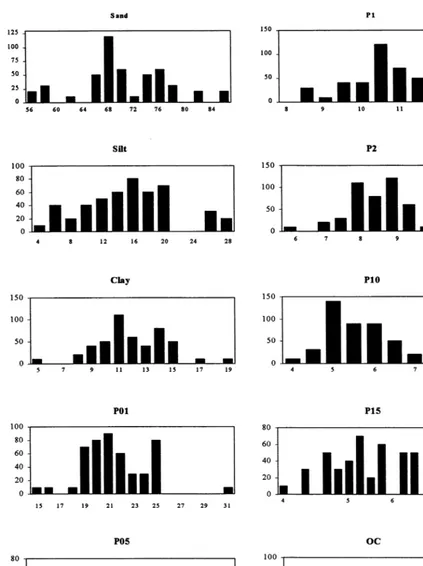
Table 1 summarizes the statistics of all mea-sured data and Fig. 1 shows the frequency distri-butions. The distributions of P01 and P2 appear somewhat bimodal, whereas the others are unimo-dal. The distributions are fairly symmetric, only P10 has skewness coefficient exceeding 1.0. How-ever, P10 was not transformed because the trans-formation to its logarithm did not change the distribution much.
The variables are generally linearly correlated; Table 2 is the correlation matrix, listing the ordi-nary product – moment correlation coefficients. Clay is correlated somewhat less strongly with all the other variables, because of its low percentages in most of the soils, and not significantly with OC. This last is only weakly and positively correlated with the variables P05, P10 and P15 and not with the others, it then seems that organic matter increases the amount of water retained as ex-pected (Reeve and Carter, 1991). All the other variables show fairly strong correlations, such as
SAND with P05 (−0.77), P10 (−0.76) and P15
(−0.76); SILT with P05 (0.74), P10 (0.74) and P15 (0.71); P01 with P05 (0.73); P05 with P10 (0.73) and P15 (0.81); P1 with P15 (0.71); P2 with P15 (0.74) and P10 with P15 (0.91). From Table 2, it is evident that all the variables are positively correlated with the others (significant
correla-Table 1
Statistical summary of the variables
P1
SAND SILT CLAY P01 P05 P2 P10 P15 OC
(g kg−1)
870.0 287.0 194.0 31.34 16.53
Maximum 13.38 12.27 9.45 7.79 13.84
9.37 6.53 5.80
Mean 711.8 162.7 125.4 22.00 13.14 11.08 7.72
9.31 6.38 5.66
Median 707.0 164.0 125.5 21.69 13.01 10.94 7.94
2.63 Skewness 0.17 0.13 −0.03 0.63
0.20
Table 2
Correlation matrix, lower trianglea
1
0.74 0.38 0.57 0.73 0.68
P10 −0.76 0.66 1
0.71 0.43 0.57 0.81 0.71
−0.76 0.74
P15 0.91 1
−0.15 n.s.
OC 0.19 n.s. −0.01 n.s. 0.17 n.s. 0.38** 0.12 n.s. 0.16 n.s. 0.33* 0.37** 1
SILT CLAY P01 P05 P1 P2 P10
SAND P15 OC
an.s., Not significant; *, significant forPB0.05; **, significant forPB0.01; all the other correlation coefficients are significant for
PB0.001.
tions) except for SAND, which is always nega-tively correlated.
Extracting the latent roots and vectors of the correlation matrix reveals the relations among the variables more clearly. Clay was eliminated from the following analysis because it is determined completely by SAND and SILT. The first three eigenvalues are listed in Table 3. The first one accounts for more than 87% of the variance, whereas the second and the third for only an additional 7 and 4%, respectively, which confirms the results of the above correlation analysis that all the variables are generally strongly correlated. In Table 4, the configuration rotated by Varimax of the first three principal components is reported with the correlation coefficients between the origi-nal variates and the principal components. The variables P01, P05 and P1, which determine the form of the soil water retention characteristic at higher water potentials, appear closely related, positively loading on the first principal compo-nent. SILT and SAND are strongly correlated with the second principal component, but in
dia-metrically opposed positions. Finally, the water contents at lower water potentials (P10 and P15) are more strongly associated with the third princi-pal component and show some link also with OC.
3.2. Spatial analysis and coregionalization
Before attempting to fit a linear model of core-gionalization, we calculated the experimental
au-tovariograms of the first three principal
components computed from the correlation ma-trix. As the first and the third principal compo-nent showed a significant trend, this last was subtracted from the values to obtain residuals, on
Table 4
Correlations between the original variates and the first three principal componentsa
aValues were multiplied by 100 and rounded to the nearest
integer. Table 3
Eigenvalues of correlatin matrix Eigenvalue
Order Percentage Accumulated percentage
1 5.80 87.37 87.37
0.51
2 7.60 94.97
Table 5
Linear equations of spatial trend for the principal components and the standardized variablesa
Principal component 1 −0.83080−0.00280×
Principal component 3 −0.8351+0.002926× −1.062+0.003722×
P01
P1 −1.034+0.003623×
−0.9924+0.003477×
P15
OC −1.355+0.004748×
aThe coefficients of the regressions are significantly different
from 0 at the probability level ofPB0.05.
Fig. 3 shows the LMC as it fits the six direct autovariograms superimposed on the experimen-tal points and Table 7 lists their coefficients. They reveal the dominant short-range autocorrelation in SAND, SILT and water content at lower
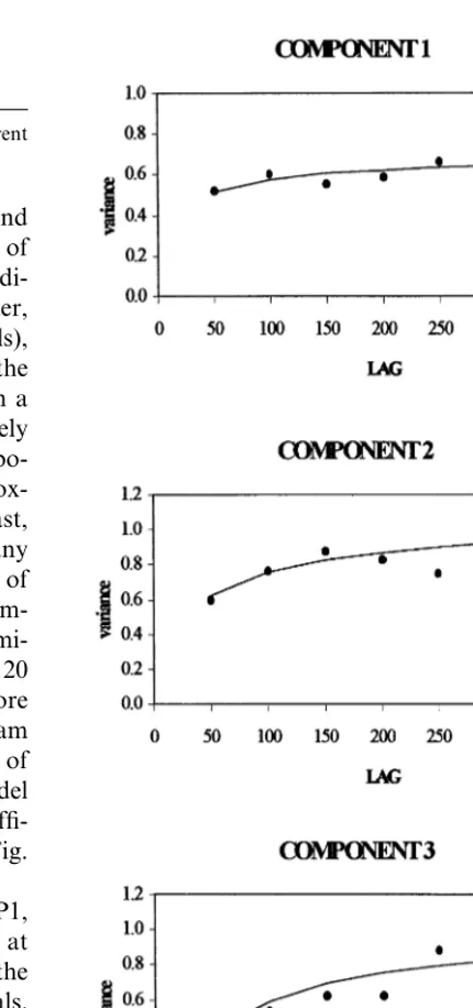
po-Fig. 2. Experimental autovariograms of the principal compo-nents plotted as points. The solid lines are those of the fitted model (LAG, m).
which the analysis was made. The linear trend equations are reported in Table 5. The presence of such a trend signifies that in well watered condi-tions the left side of the field is probably moister, whereas under dry conditions (smaller potentials), larger water contents are likely to be found in the right half of the field. This may be explained in a greater concentration of organic matter (positively correlated with the water content at smaller po-tentials) in the right side of the field in the prox-imity of the sites of slurry discharge. In contrast, texture (second component) does not show any significant spatial trend, at the probability level of PB0.05. The three graphs of the principal
com-ponents (Fig. 2) display a steady increase in semi-variance with increasing lag distance to about 120 m, then reach a maximum more slowly at more than 300 m. To represent the whole variogram with both short- and long-range structures, of each PC, we fitted a double exponential model with a nugget (Eq. (1)). The values of the coeffi-cients are given in Table 6. The solid lines in Fig. 2 represent these fitted models.
Some of the standardized variables (P01, P1, P15 and OC) showed a significant linear trend at the probability level ofPB0.05 (Table 5), and the
Table 6
Coefficients of double-exponential model fitted to the principal components C1
C0 C2 a1(m) a2(m)
1.18×10⁻¹ 2.03×10⁻¹
Principal component 1 3.38×10⁻¹ 40 1.17×10²
Principal component 2 3.00×10⁻¹ 1.53×10⁻¹ 4.98×10⁻¹ 40 1.17×10²
1.55×10⁻² 7.71×10⁻¹ 40 1.17×10²
9.09×10⁻²
Principal component 3
Table 7
Coefficients,bk, of double-exponential coregionalization model for standardized direct variograms
SILT P01 P1 P15
SAND OC
0.214 0.468 0.677 0.094
0.225 0.260
Nugget,b1
0.858
Short range,b2 0.987 0.221 0.147 1.074 0.234
Long range,b3 0.420 0.103 0.523 0.024 0.176 0.703
P01–SAND P01–SILT P1–SAND P1–SILT P1–P01
SAND–SILT P15–SAND
−0.204 0.093 −0.321
Nugget −0.184 0.196 0.391 −0.058
−0.434 0.466 −0.349 0.373
−0.920 0.174
Short range −0.938
Long range −0.185 −0.207 0.186 0.100 −0.045 −0.052 0.041 P15–P01 P15–P1 OC–SAND OC–SILT OC–P01
P15–SILT OC–P1 OC–P15
0.162 0.193 0.021
Nugget −0.002 0.001 0.111 −0.079 0.035
0.465 0.397 −0.059 0.074
0.999 0.048
Short range −0.009 −0.043
−0.289 0.011 0.017 −0.130
Long range −0.079 −0.552 0.007 0.349
tentials (P15). On the contrary, organic carbon dominates the long-range structure.
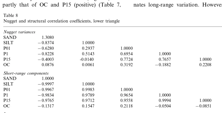
The short-range structure dominates the cross-correlations between SAND and SILT (negative), P15 and SAND (negative) and P15 and SILT (positive), whereas the long-range structure domi-nates mainly that of OC and P01 (negative) and partly that of OC and P15 (positive) (Table 7,
cross-variograms not reported). The importance of each structure reflects the influence of the corresponding spatial variable or pair of variables on soil variation. Therefore, texture and soil water content at lower potentials control spatial varia-tion at short-range, whereas organic carbon in interaction with soil water characteristic domi-nates long-range variation. However, the whole
Table 8
Nugget and structural correlation coefficients, lower triangle Nugget6ariances
1.3080 SAND
SILT −0.8374 1.0000
−0.6280 0.2937 1.0000
P01
P1 −0.8228 0.5143 0.6954 1.0000
0.7724 0.7657 1.0000
OC 0.0061 −0.1882 0.2208 1.0000
Short-range components
SAND 1.0000
SILT −0.9997 1.0000
1.0000
P01 −0.9967 0.9983
0.9789
−0.9834 0.9654 1.0000
P1
−0.9765 0.9712 0.9558
P15 0.9994 1.0000
−0.1317 1.0000
OC 0.1547 0.2118 −0.0504 −0.0851
Long-range components
SAND 1.0000
−0.8911 1.0000 SILT
P01 −0.4422 0.8011 1.0000
0.9997
P1 −0.9019 −0.4640 1.0000
−0.5846 0.1528
P15 −0.9539 0.1769 1.0000
−0.9107 0.0566 0.9927
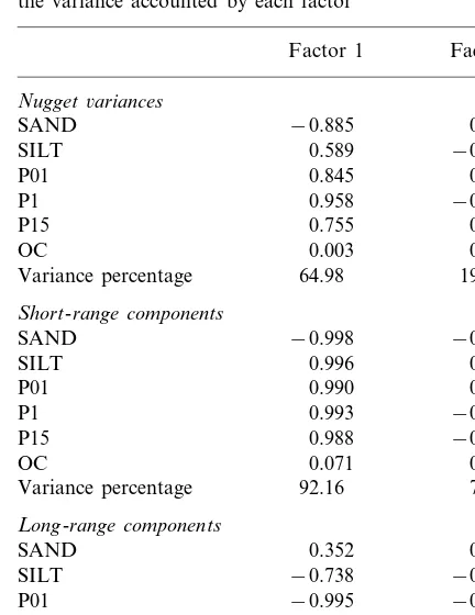
Table 9
Correlations between the original variables and the first two regionalized factors for each spatial scale and percentage of the variance accounted by each factor
Factor 2 Factor 1
Nugget6ariances
SAND −0.885 0.218
−0.282
Short-range components
−0.998
Long-range components
0.936
charge, can modify water retention processes in the soil.
Another way to envisage spatial correlations is to estimate the principal components of the core-gionalization matrices (regionalized factors). The correlations between the original variables and the regionalized factors are reported in Table 9. Except for the nugget, the first two regionalized factors explain the actual total variance either at short- or long-range scale. Because nugget variance is likely to represent not only mainly microscale variance (B50 m), but also embraces procedural errors, we
preferred to restrict our discussion of the results to the short and long-range components of the vari-ance. The first factor of the short-range component (effective range, 120 m) explains 92% of the overall variation at this scale and is very strongly corre-lated with soil texture (negatively with SAND and positively with SILT) and positively with the soil water characteristic. The second factor at the same spatial scale accounts for the remaining 8% of the variance and is strongly and positively correlated with OC. At this scale, textural and water retention characteristics dominate spatial variation and do not seem sensitively influenced by the presence of organic carbon, as it was previously reported.
The first factor of the long-range component (effective range, 350 m) explains 73% of the vari-ance and is positively correlated with OC and P15 and negatively with P01 and SILT. At this scale then organic carbon shows a strong and positive correlation with soil water content at smaller poten-tials and a negative correlation with water content at larger potentials and with the finer components of texture. The second factor of the long-range
component accounts for 27% and is positively
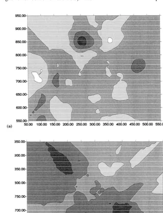
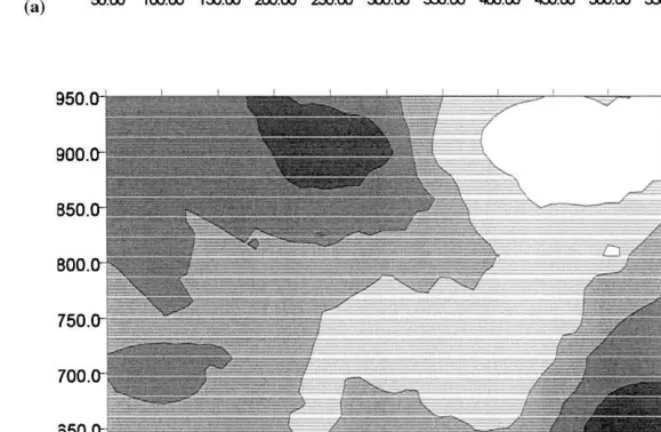
correlated with coarser elements of soil texture and water content at intermediate water potentials (P1). The cokriged maps of the first and the second regionalized factors at short-range scale (Fig. 4a and Fig. 5a) look similar enough, with some patches in the field (light zones) corresponding to larger concentrations of silt (first factor), very often associated also with greater concentration of or-ganic carbon (second factor). These zones comprise the localized positive effects of slurry discharge on OC concentration and are also wetter both in dry and well-watered conditions.
dis-At long-range scale, the maps of the first and the second regionalized factors (Fig. 4b and Fig. 5b) look less uniform, with light areas for the first factor characterized by greater concentration of organic carbon associated with wetter soil at smaller potentials. OC tends to accumulate in the preferential sites for slurry discharge (the large area in the right lower corner of the field). The
long-range map of the second factor (Fig. 5b) reveals a well-defined gradient of texture along the direction NW – SE — sand concentration in-creases from the corners to the center of the field. Therefore, the wide zone of greater concentration in organic matter, observed in the lower right corner, is connected with the larger silt concentra-tions. It needs to be pointed out that here the soil
Fig. 5. Co-kriged maps of the second regionalized factor at short- (a) and long- (b) range spatial scale (abscisse and ordinate, m).
could be locally naturally slow to water infiltra-tion. So, it was necessary to be judicious in adding slurry that could introduce hydrophobic tenden-cies not to unduly aggravate this natural property of the soil. European Community regulations rec-ommend organic matters applications in order to ensure adequate plant nutrients and to hold down heavy metal contamination. We would advise
first of all, to the improvement of the pore system in soil (Pagliai and Vignozzi, 1998), which leads to better soil structure, but also to the water adsorp-tion capacity of organic matter (Metzeger and Yaron, 1987).
4. Conclusions
The results of this study support the following conclusions:
the short-range spatial component represents
mainly the texture and soil water characteris-tics. At this scale, organic carbon does not seem to be correlated with the water retention characteristics of the soil, even if higher OC concentrations are generally associated with larger proportions in silt and water;
organic carbon behaves differently at
long-range scale (120 – 350 m) — at these distances, it is strongly and positively correlated with soil water content at lower water potential (P15), but negatively correlated with water content at higher water potential (P01). It would then seem that the discharge of liquid manure on the soil produced a significant effect at longer spatial scale, modifying the water holding ca-pacity in two distinct ways. The first one is a direct effect due to the inclusion of organic particles with a large capacity to adsorb water, increasing the total amount of water retained by the soil. The second effect is somewhat indirect, because the inclusion of organic mat-ter increases soil porosity, in our case mostly increasing the number of pores sized about 0.2 – 0.5mm corresponding to the smaller water potentials. This may be associated with in-creases in the proportion of larger size aggre-gates at the expense of smaller aggreaggre-gates. However, it is also possible that the hydropho-bicity of manure may have greatly decreased the rate of water entry into larger size aggre-gates (negative correlation between OC and P01);
geostatistical analysis might then prove useful
in describing the impact of liquid manure dis-charge on the soil water retention characteris-tics and in delineating areas with higher
concentrations of organic matter. It might also be used as a tool in decision-making often aimed at delineation of areas targeted at reme-diation or additional sampling. Moreover, such an analysis allows to assign scores to areas with different susceptibility to liquid manure dis-charging on the basis of their pedological con-ditions; and
finally, multivariate geostatistical techniques
such as FKA are suitable for distinguishing the different processes causing spatial variation at different scales. The method provides quantita-tive measures of complex interactions between soil properties and may then be particularly useful for formulating hypothesis on what spe-cifically caused the variability. In this way, it is possible a better management of spatial and temporal variability associated with all aspects of agricultural production for the purpose of improving crop performance and environmen-tal quality.
References
Borges, R., Mallarino, A.P., 1997. Field-scale variability of phosphorus and potassium uptake by no-till corn and soybean. Soil Sci. Soc. Am. J. 61, 846 – 853.
Cahn, M.D., Hummel, J.W., Brouer, B.H., 1994. Spatial anal-ysis of soil fertility for soil-specific crop management. Soil Sci. Soc. Am. J. 58, 1240 – 1248.
Castrignano`, A., Mazzoncini, M., Giugliarini, L., 1998. Spa-tial characterisation of soil properties. Adv. Geoecol. 31, 105 – 111.
Castrignano`, A., Giugliarini, L., Martinelli, P., Risaliti, R., 2308. Study of spatial relationships among soil physical – chemical properties using multivariate geostatistics. Geo-derma (in press).
Davidoff, B., Selim, H.M., 1988. Correlation between spatially variable soil moisture content and soil temperature. Soil Sci. Soc. Am. J. 145, 1 – 10.
Deutsch, C.V., Journel, A.G., 1998. GSLIB: Geostatistical Software Library and User’s Guide. Oxford University Press, New York.
Dobermann, A., Goovaerts, P., George, T., 1995. Sources of soil variation in an acid Ultisol of the Philippines. Geo-derma 68, 173 – 191.
Dobermann, A., Goovaerts, P., Neue, H.N., 1997. Scale-de-pendent correlations among soil properties in two tropical lowland rice fields. Soil Sci. Soc. Am. J. 61, 1483 – 1496. Goovaerts, P., 1992. Factorial kriging analysis: a useful tool
Goovaerts, P., 1997. Geostatistics for Natural Resources Eval-uation. Oxford University Press, New York.
Goovaerts, P., Webster, R., 1994. Scale dependent correlation between topsoil copper and cobalt concentrations in Scot-land. Eur. J. Soil Sci. 45, 79 – 95.
Goulard, M., Voltz, M., 1992. Linear coregionalization model: tools for estimation and choice of cross variogram matrix. Math. Geol. 24, 269 – 286.
Matheron, G, 1982. Pour une analyse krigeante des donne´es regionalise´es. Report N-732, Centre de Geostatistique, Fontainebleau.
Metzeger, L., Yaron, B., 1987. Influence of sludge organic matter on soil physical properties. Adv. Soil Sci. 7, 141 – 163.
Pagliai, M., Vignozzi, N., 1998. Use of manures for soil improvement. In: Wallance, A., Terry, R.E. (Eds.), Hand-book of Soil Conditioners. Marcel Dekker, New York. Reeve, M.J., Carter, A.D., 1991. Water release characteristic.
In: Smith, K.A., Mullins, C.E. (Eds.), Soil Analysis. Marcel Dekker, New York, pp. 111 – 160.
Stafford, J.V., Ambler, B., Lark, R.M., Catt, J., 1996. Map-ping and interpreting the yield variation in cereal crops. Comput. Electron. Agric. 14, 101 – 119.
Vargas-Guzman, J.A., Warrick, A.W., Myers, D.E., 1999a. Scale effect on principal component analysis for vector random functions. Math. Geol. 31 (6), 701 – 722. Vargas-Guzman, J.A., Warrick, A.W., Myers, D.E., 1999b.
Multivariate correlation in the framework of support and spatial scales of variability. Math. Geol. 31 (1), 85 – 103. Wackernagel, H., 1989. Description of a computer program
for analyzing multivariate spatially distributed data. Com-put. Geosci. 15, 593 – 598.
Wackernagel, H., 1994. Cokriging versus kriging in regional-ized multivariate data analysis. Geoderma 62, 83 – 92. Webster, R., Atteia, O., Dubois, J.P., 1994. Coregionalization
of trace metals in the soil in the Swiss Jura. Eur. J. Soil Sci. 45, 205 – 218.
West, C.P., Mallarino, A.P., Wedin, W.F., Marx, D.B., 1989. Spatial variability of soil chemical properties in grazed pastures. Soil Sci. Soc. Am. J. 53, 784 – 789.