www.elsevier.comrlocatereconbase
Empirical tests of efficiency of the Italian index
options market
Laura Cavallo
a,b,), Paolo Mammola
c,1a
Prime Minister’s Office, Rome, Italy b
UniÕersity of RomeATor Vergata,B Rome, Italy
c
Citibank Milan, N.A. Foro Bonaparte 16-20123 Milan, Italy
Accepted 9 May 2000
Abstract
The purpose of this paper is to investigate whether the Italian index option contract
ŽMIBO30 , recently introduced in the Italian Derivatives Market IDEM , is efficient. Two. Ž .
different methods are used in the analysis. First, we tested on the Italian index option market the validity of the put–call parity conditions, extended to account of transaction costs associated with replicating and establishing a short hedge on the index. We find that the significant deviations from put–call parity are not exploitable when all transaction costs are accounted for. Since the put–call parity is just a weak test for market efficiency, we further investigate the possibility to generate profitable positions through the simulation of an ex-post volatility hedging strategy. This strategy does not allow for systematic abnormal returns, supporting the hypothesis that option prices are consistent with market efficiency.
q2000 Elsevier Science B.V. All rights reserved.
JEL classification: G13; G15
Keywords: Lower-boundary; Put–call parity; Volatility trading; Implied volatilities; Transaction costs
)Corresponding author. Department of Economic Affairs, Prime Minister’s Office, via Barberini 47,
00187 Rome, Italy. Tel.:q39-347-6079633; fax:q39-06-23313148.
Ž . Ž
E-mail addresses: [email protected] L. Cavallo , [email protected] P. Mam-.
mola .
1
Tel. :q39-335-5827738; fax :q39-02-86474362.
0927-5398r00r$- see front matter q2000 Elsevier Science B.V. All rights reserved.
Ž .
1. Introduction
The Italian option on index MIB30 contract or AMIBO30B introduced in the
Ž .
Italian Derivatives Market IDEM on November 1995 represents one of the most important steps aimed to improve the efficiency and the liquidity of the Italian financial markets. Trading on the IDEM started on November 1994 with the introduction of the future contract on the same index, the Mib30. The strong success of this contract, which enjoyed a rapid development and is now placed among the five most traded future contracts in Europe, convinced the Italian Authorities to introduce an option contract on the index, the MIBO30, and later on Žin February 1996 on single stocks, the ISO. a. This paper contains an empirical analysis directed towards an investigation of whether the MIBO30 option market is efficient.
For the purposes of this study, the market is efficient if it does not present arbitrage opportunities. Since Black and Scholes published their article on option pricing in 1972, several theoretical and empirical works have been written on option pricing. However, most of these studies have been conducted on the Chicago Board Option Exchange and very few studies have been undertaken to test the efficiency of other option markets. In particular, the Italian Option market is quite recent and is scarcely investigated2.
To analyse the efficiency of the Italian Index Option Market, the Black and
Ž .
Scholes 1971,1972 model is probably the simplest valuation model, and evidence from dealers operating in the market indicates that it is widely used. However, there are several problems in carrying out empirical research based on the Black–Scholes as on any option pricing models. The first problem is that any statistical hypothesis about how options are priced has to be a joint hypothesis to
Ž . Ž .
the effect that i the model is valid and ii markets are efficient. To distinguish between the two hypotheses of market efficiency and model validity, one of the two has to be taken as an assumption. A second problem concerns the choice of the best estimate of stock price volatility. A third problem is to ensure that data on the stock price and option price are synchronous.
The current study attempts to overcome the above difficulties in three substan-tive ways. First of all, it uses a very high quality data source, which contains not only transaction prices but also quoted bid and ask prices. Second, in the first part of the work it employs a test of market efficiency, the put–call parity test, which do not rely for its validity on the restrictive Black–Scholes assumptions. More-over, this test can easily be manipulated and extended to take account of the
2 Ž .
Two previous studies Barone and Cuoco, 1989, 1991 investigated the premium contracts on the Italian stock exchanges. Trades on premium contracts were substituted by trades on options few months
Ž .
after the introduction of contracts. For an analysis of the MIBO30 see Cavallo 1998 and Cavallo et al.
frictions of the market such as transaction costs, so that new conditions are derived and subjected to empirical test. Since the put–call parity is only a weak test of market efficiency, results obtained are further investigated in the second part of the work, where an ex-post hedging strategy is simulated to verify the possibility to exploit the mispricing evidenced by comparing actual option prices with Black– Scholes prices. This dynamic hedging strategy, taking into account transaction costs and relaxing some of the assumptions of the Black–Scholes model, allows verification of the hypothesis that mispricings are due to an inaccuracy of the model rather than to the inefficiency of the market.
The paper is organised as follows. Section 2 describes the Italian option market and the data set used. In Section 3, the put call parity conditions in the presence of transaction costs are derived and subjected to empirical test on the Italian market using infra-day synchronous option and index prices. In Section 4, different measures of volatility are derived and used to simulate a volatility trading strategy, in order to verify the possibility to realise systematic abnormal returns on the Italian option market. Some concluding remarks are offered in Section 5.
2. Market and data
2.1. The AMIBO30B market
The empirical tests of this work are based on data on index options, MIBO30, recently introduced in the IDEM. The index option contracts traded on IDEM are based on the MIB30 index, which has been proven to be a reliable indicator of the Italian market. The MIB30 index is a capitalisation-weighted index that comprises the 30 most liquid and highly capitalised shares traded on the Italian market. The shares in the index account for over 72% of total market capitalisation, and almost
Ž .
75% of trading volume. Its correlation with the Italian general index MIB is above 0.99. The contract size is set at 10 000 ITL for each point of the index. MIB30 options are European style, which means they can only be exercised at expiration. The options have cash settlement.
At any given time there are options available for at least five expiration dates: Ž
the three nearest expirations dates of the quarterly cycle March, June, September .
and December , which correspond to the expiration dates of the future contract, Ž
and the two nearest monthly expirations a monthly expiration corresponds to one .
2.2. Data and methodological issues
In this section we describe and motivate some methodological issues used in the analysis. The empirical tests were carried out only on options with a maturity of 1 month. The main reason of this choice is that the market is still very young and the thinness of trading makes prices on other expirations not representative.
Ž .
The risk-free rate was estimated by the European interbank offered rate Euribor published daily by the Sole 24 ore.3 This is the same interest rate used by the
Ž .
CONSOB the Italian Securities and Exchange Commission to vigil the daily behaviour of option prices and the behaviour of market makers in setting the bid and ask quotations. It is then likely that market makers refer to this interest rate in order to verify whether their quotations are consistent with the theoretical value of the option. The value of the Euribor published in the Sole 24 ore is the ask rate;
Ž .
the bid interest rates can be obtained subtracting 1r8 0.125% from the ask rates. We eliminated options with fewer than seven calendar days to expiration. Most dividend payments of the stocks included in the index are concentrated in the months of May and June. However, since dividend payments occur after the expiration day of the option, they do not affect the options with 1-month maturity used for the empirical tests.
When, as in our case, the underlying security is not a single option but an index, arbitrageurs face two alternatives: replicate a portfolio representative of the
Ž .
securities included in the index, or use the futures on the index Fib30 . We decided to use the first alternative and to replicate the index. Although this choice may appear more costly, it must be noticed that using the future the trader would incur the Abasis risk,B when the expiration of the future does not correspond to that of the option. Moreover, the MIB30 index includes only 30 securities and is not very difficult to replicate. The high movements observed in the prices of the securities included in the index in proximity to the maturity of the options support the assumption that replicating the index is a common practice among traders. Another issue accounted for in the analysis is the cost of short selling the index. If the arbitrage involves a short hedge in the index, the arbitrageur should assume a further cost represented by the cost of securities lending. The market for securities lending in Italy is an Over the Counter Market. The characteristics of the contracts are not standardised and can be designed to best satisfy the necessities of the
4 Ž .
arbitrageur. Because data on the securities lending market interest rates repo are
3
To match the interest rate to the period of expiry of the options, we used a Relevant Interest Rate obtained by linear interpolation of interest rates for different time horizons.
4
Ž .
not available for it is an OTC market , for the empirical tests we used as a proxy the AbidB interest rate. We also account for costs due to the cash settlement procedure, which distinguish index option from stock and commodities option. The only relevant difference in the results is that the trader has to pay the additional commission cost to close on the market at maturity the position open on the underlying asset.
3. Put–call parity and transaction costs
In this section, the put–call parity conditions are derived and subjected to empirical testing on data on index options traded on the IDEM.
The data used to test the put–call parity conditions consist of infra-day prices, captured every 15 min from 10 a.m. to 5.30 p.m. from July 29, 1996 to February 18, 1997 for a total of 3642 observations. Data include ask price, bid price and
Ž .
transaction price of at the money options call and put and on the MIB30 futures. In our study, we estimated the MIB30 bid and ask prices applying to the transaction price the same spread observed for the future on the index MIB30.5
Ž .
The put–call parity model was first developed by Stoll 1969 , and then
Ž .
extended and modified by Merton 1973 . The well-known basic put–call parity condition, when there is no dividend payment, is the following:
CsPqSyKeyrŽTyt..
Ž .
1Ž .
The non-arbitrage conditions can be derived from Eq. 1 establishing two portfolios, both of which result in zero pay-off at expiration. The first portfolio represents a long-hedge position, because it involves taking a long position in the underlying share. The second portfolio represents a short-hedge position. In the absence of dividends and transaction costs, those conditions are, respectively:
CyPySqKeyrŽTyt.F0,
Ž .
2PyCqSyKeyrŽTyt.F0.
Ž .
3Tests based on the put–call parity conditions, though weak tests of market efficiency, have been widely used in the empirical literature. Some of these studies
Ž .
basically supported the theory Nisbet, 1992; Klemkosky and Resnick, 1979 , but Ž
some inefficiency where also found to exist Stoll, 1969; Gould and Galai, 1974; .
Evnine and Rudd, 1985; Finucane, 1991 .
5
In this section, we extend the put–call parity conditions to take into account frictions not considered in previous tests, in particular, the costs of replicating the index and the cost of short selling. Since the option selected for the analysis are the most liquid and the spread is precisely bounded by the Italian market regulation, we may be confident that the bid and ask prices used to account for the spread effectively corresponds to a transaction.6 The availability of infra-day prices ensures a good synchronisation between the option prices and the underly-ing security. Since the Italian Market trades are matched in real-time by the electronic trading system, it is reasonable to assume that the arbitrage strategy could be implemented at the same prices prevailing when the profit opportunity were identified. This allows to overcome one of the main problems related to put–call parity tests, that is the possibility that prices used to identify the arbitrage opportunity do not represent tradable prices. The put–call parity conditions are
Ž Ž ..
obtained as follows. If the expression representing a long hedge Eq. 2 is not verified, a profit can be made by purchasing the index at its ask price, the put at its ask price, and selling the call at its bid price. The initial investment can be
Ž . financed at the risk free rate. In the case of a short hedge, if condition 3 is not verified, the strategy to profit from the mispricing consists in buying the call, selling the put and short selling the portfolio which replicate the index. Accounting for all transaction costs involved in the implementation of these strategies, the non-arbitrage conditions become, respectively, for a long and a short hedge:
C yP yI qKeyrŽTyt.
where: TCwc and TCwp are, respectively, the cost of writing a call or a put; TCbc and TCbp are the cost of purchasing the call or the put; TCbi and TC are the costsi
Ž
of purchasingrselling the index when the position is closed at maturity T we .
calculate the present value of the commission cost and Tk are the clearing commission on the option, usually very small and omitted from the empirical tests. Note that in the short-hedge condition the present value of K is calculated
Ž .
using the repo rp rate. This allows accounting for the assumption that the cost of the trading will be financed by the funds deposited with the lender of the securities.
6 Ž .
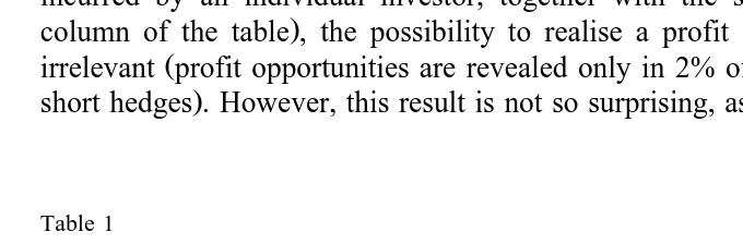
Table 1 summarises the results of the put–call parity tests under different hypothesis about transaction costs. Cases I and II represent the tests conducted using, respectively, transaction prices and the bid and ask prices. For both cases I and II, the table reports three columns with the results obtained under three different assumptions on the level of commission costs. In the first column, to make the results comparable with studies that ignore transaction costs, these costs
Ž .
were omitted Tcs0 . In the second and the third column, we considered the level of transaction costs incurred, respectively, by an occasional investor and by an arbitrageur. The position of an arbitrageur involves a lower level of transaction costs.
Referring to the average market commission, for an option contract we used a transaction cost of 10 000 ITL for the arbitrageur and 15 000 ITL for an individual investor. Commissions on replicating the index are expressed in index points, and are 5 and 10 index points, respectively, for an arbitrageur and an individual investor. Clearly, the larger the transaction costs, the wider the band within which prices can fluctuate without creating arbitrage opportunities.
Consistently with expectations, the number of hedges, which would have provided a profit opportunity decreases substantially when commission costs and the bid ask spread are included. When we consider the level of transaction cost
Ž incurred by an individual investor, together with the spread bid–ask the last
.
column of the table , the possibility to realise a profit from the hedge become Ž
irrelevant profit opportunities are revealed only in 2% of the simulated long and .
short hedges . However, this result is not so surprising, as this is only a weak test
Table 1
Number and average values of profitable hedges for cases I and II and different levels of transaction costs
Profitable hedges Case I — transaction prices Case II — bra spread Tcs0 TcsTc1 TcsTc2 Tcs0 TcsTc1 TcsTc2
Long hedge Number 1798 1078 546 589 213 82
% of the sample 49 30 15 16 6 2
)
Average value 19.4 16.34 16.23 13.04 14.45 20.11
z 43.9 27.55 16.94 18.91 9.698 6.576
Short hedge Number 1780 1083 596 519 193 70
% of the sample 49 30 16 14 5 2
Average value 20.65 18.34 18.33 13.62 15.67 23.71
z 43.7 29.95 20.8 16.03 8.387 5.567
Case I: Long hedge: CyPyIqKeyrŽTyt.FTc; Short hedge: PyCqIyKeyr pŽTyt.FTc; Case
II: Long hedge: C yP yI qKeyrŽTyt.FTc; Short hedge: P yC qI yKeyr pŽTyt.F
bid ask ask bid ask bid
Tc; where Tc is the total transaction cost. In the first column of the table, Tcs0, in the second column Tc1 represents the lower transaction cost level incurred by an arbitrageur, in the third column Tc2 is the transaction cost incurred by an individual investor.
)
of market efficiency. What is interesting to note in the results is that, in contrast
Ž . Ž .
with the findings of Klemkosky and Resnick 1980 on CBOE and Nisbet 1992
Ž .
on the London Traded Option Market LTOM , we do not observe a larger number of profitable short hedges than profitable long hedges. Different elements can
Ž .
contribute to interpret this result: i in contrast with other markets, in the Italian Ž Market it is not particularly difficult or costly to establish short hedge positions at
. Ž .
least for the 30 stocks which constitute the index ; ii previous studies of put call parity, including the ones mentioned above, have not explicitly allowed for transaction costs associated with the securities lending market when the strategy involve a short position in the underlying security. Another explanation is that market makers and options dealers prefer trading on the future contract on the MIB30 index rather than short selling the portfolio, which replicates the index. Moreover, the main insight we can derive from the way we presented the results is that tests of market efficiency critically depend on the treatment of transaction costs. This is particularly true for tests based on an option-pricing model, which rely for their validity on continuous portfolio rebalancing. This problem will be investigated further in Section 4, where a stronger test of market efficiency is implemented.
4. Volatility trading and market efficiency
4.1. TheÕolatility trading strategy
The objective of this analysis is to test the efficiency of MIBO30 prices, through the implementation of a volatility trading strategy attempting to exploit deviations between actual option prices and theoretical prices. More precisely, a volatility trading consists of formulating trading strategies on the basis of one’s own anticipation of the future volatility of the security underlying the option
Ž .
contract. To expect a future volatility higher lower than that currently registered
Ž .
on the market, corresponds to foreseeing a rise lowering in the price of the
Ž .
options. The related strategy consists in purchasing selling the options.
The first studies aimed at verifying the efficiency of the options market based on an analysis of the deviations between theoretical and effective prices were
Ž . Ž .
conducted by Black and Scholes 1972 , Galai 1977 , and MacBeth and Merville Ž1979 . These authors examined the possibility of realising above-normal returns.
Ž
by purchasing optionsAundervaluedB by the market under the assumption that the .
Ž . possibility of realising such extra-returns. A study of Joo and Dickinson 1993 analyses the efficiency of the European Option Market, developing a dynamic hedging strategy that takes into account the effects of bid and ask spread costs.
Ž .
A study of Xu and Taylor 1995 examines the conditional volatility and the informational efficiency of currency options.
4.2. Data andÕolatility estimates
A sample consisting of daily data was used for the present analysis. This sample differs from the one used to test the put–call parity condition, not only for the period and the frequency of the data, but also because in this sample, apart from Aat-the-moneyB options, also AinB and Aout-of-the-moneyB options are available. The period surveyed is from December 1996 to September 1997. Synchronisation is essential to obtain an accurate estimate of the implied volatility and to avoid distortion of the results of the hedging simulations. This is the reason why this sample has been constructed through a very accurate and time-consuming procedure. From the data on the index, available minute by minute, we selected the price at the same time every day. On a daily basis, from the set of prices of all put and call options contracts effectively concluded, continuously quoted, we
Ž
selected options with three different strike price values the strikes at-the-money, .
in-the-money and out-of-the-money closest to the central strike concluded as close as possible to the time the index was selected.7
The dynamic strategy was repeated using historical and implied estimates for
Ž .
future volatility. The historic volatility or Historic standard deviation, Hsd was estimated as the moving average of standard deviation of the logarithmic differ-ences in the index daily prices. The estimation period is 20 days, which corre-sponds to the forecast period, the option time to maturity, measured in trading days.8Annual measures of volatility are obtained multiplying the daily values of
'
the standard deviations by 250 .7 Ž .
Harvey and Whaley 1991 suggest that the use of more than one value for every day partly mitigates distortion of the estimate of volatility due to considering the effective transaction prices, ignoring the bid and ask prices. In order to reduce measurement errors, we selected also a second observation every day to use to calculate implied volatilities. Calculating implied volatilities using call and put prices on several strikes, in turn calculated as the average of two daily values, we believe that we have considerably reduced the measurement problems evidenced by Harvey and Whaley.
8
The opportunity to utilise trading days rather than calendar days when calculating volatility is
Ž .
Implied volatility estimates are obtained as a weighted average of single
Ž .
implied volatilities. Following Chiras and Manaster 1978 , the weights used are the elasticity of the individual prices to volatility:
n EW s
where WISD is theAWeighted Implied Standard DeviationB for the index Mib30 on the observation date, ISD thej AImplied Standard DeviationB of option j, W is
Ž .Ž .
the option price and dWjrdsj sjrWj is the price elasticity of option j with Ž .
respect to the index standard deviation s . We calculated three measures of
Ž .
implied volatility: the first WISDc is constructed using the three call option
Ž . Ž .
prices respectivelyAatB, AinB andAoutB of the money . The second WISDp is
Ž .
computed using the three put option prices. The last WISDpc is a weighted average of the first two. Some descriptive evidence on the time series properties of the implied volatilities is provided in Table 2.
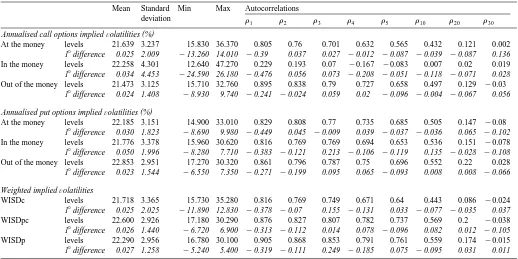
All implied volatilities evidence persistence in the level of volatility, all the series presenting significant positive serial correlation.9 The decline of autocorrela-tions at longer lags is an indication of stationarity. Looking at differenced series, estimated coefficients show negative serial correlation at lag 1 for all implied
Ž .
volatility estimates. This result, consistent with the findings of French et al. 1987
Ž .
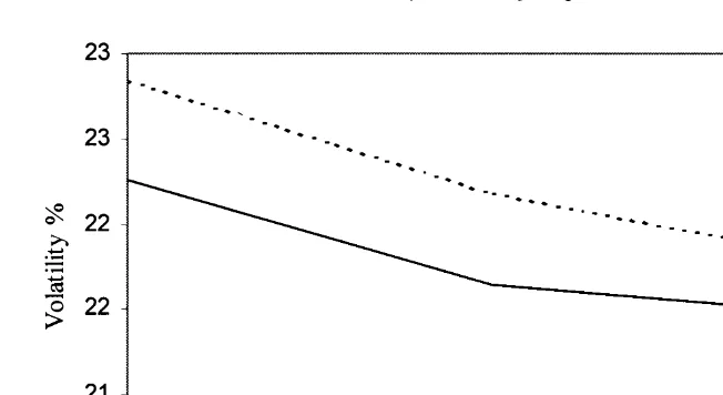
on S & P 500 volatility and Harvey and Whaley 1992 on S & P 100 index options, may indicate mean reversion and predictability in volatility changes.10 The table shows that the average implied volatilities of the calls are always significantly lower than the average volatilities of the puts.11 This result, also evidenced in Figs.
Ž .
1 and 2, is consistent with the finding of Harvey and Whaley 1992 on implied
Ž .
volatilities of S & P100 index options, and of Gemmill 1996 on implied volatili-ties of the FTSE 100 index options. Fig. 1 presents the smile of implied volatilivolatili-ties from call and put options. Both smiles show a left-skewed pattern around the
Ž .
at-the-money strike price k . This result is consistent with expectations,
con-firmed by the literature on asymmetric GARCH models: as the market falls, stock
9
We can observe that the implied volatility series derived from in the money call options presents a sensibly lower level of autocorrelation, which tend to disappear at lag 3. A possible explanation is that in the money call options are more likely to be affected by measurement problems, as we will precise in discussing volatility trading strategy results.
10 Ž .
Harvey and Whaley 1992 underline that negative serial correlation is only a weak evidence against the hypothesis that volatility changes are unpredictable. In fact, it may be spuriously induced by asynchronous observation of the index and the option and by the bid ask spread.
11
()
Summary statistics and autocorrelations for the index MIB30 options implied annualised volatilities, based on daily data for the period December 1996, through September 1997
Mean Standard Min Max Autocorrelations
deviation r r r r r r r r
1 2 3 4 5 10 20 30
( ) Annualised call options impliedÕolatilities %
At the money levels 21.639 3.237 15.830 36.370 0.805 0.76 0.701 0.632 0.565 0.432 0.121 0.002
18difference 0.025 2.009 y13.260 14.010 y0.39 0.037 0.027 y0.012 y0.087 y0.039 y0.087 0.136
In the money levels 22.258 4.301 12.640 47.270 0.229 0.193 0.07 y0.167 y0.083 0.007 0.02 0.019
18difference 0.034 4.453 y24.590 26.180 y0.476 0.056 0.073 y0.208 y0.051 y0.118 y0.071 0.028
Out of the money levels 21.473 3.125 15.710 32.760 0.895 0.838 0.79 0.727 0.658 0.497 0.129 y0.03
18difference 0.024 1.408 y8.930 9.740 y0.241 y0.024 0.059 0.02 y0.096 y0.004 y0.067 0.056 ( )
Annualised put options impliedÕolatilities %
At the money levels 22.185 3.151 14.900 33.010 0.829 0.808 0.77 0.735 0.685 0.505 0.147 y0.08
18difference 0.030 1.823 y8.690 9.980 y0.449 0.045 y0.009 0.039 y0.037 y0.036 0.065 y0.102
In the money levels 21.776 3.378 15.960 30.620 0.816 0.769 0.769 0.694 0.653 0.536 0.151 y0.078
18difference 0.050 1.996 y8.280 7.710 y0.383 y0.121 0.213 y0.106 y0.119 0.135 y0.028 y0.108
Out of the money levels 22.853 2.951 17.270 30.320 0.861 0.796 0.787 0.75 0.696 0.552 0.22 0.028
18difference 0.023 1.544 y6.550 7.350 y0.271 y0.199 0.095 0.065 y0.093 0.008 0.008 y0.066 Weighted impliedÕolatilities
WISDc levels 21.718 3.365 15.730 35.280 0.816 0.769 0.749 0.671 0.64 0.443 0.086 y0.024
18difference 0.025 2.025 y11.890 12.830 y0.378 y0.07 0.155 y0.131 0.033 y0.077 y0.035 0.037
WISDpc levels 22.600 2.926 17.180 30.290 0.876 0.827 0.807 0.782 0.737 0.569 0.2 y0.038
18difference 0.026 1.440 y6.720 6.900 y0.313 y0.112 0.014 0.078 y0.096 0.082 0.012 y0.105
WISDp levels 22.290 2.956 16.780 30.100 0.905 0.868 0.853 0.791 0.761 0.559 0.174 y0.015
18difference 0.027 1.258 y5.240 5.400 y0.319 y0.111 0.249 y0.185 0.075 y0.095 0.031 0.011
Weights used to calculate weighted implied volatilities are the elasticities of the single options to volatility. WISDc and WISDp are obtained, respectively,
Ž .
Fig. 1. Volatility smiles. The figure evidences the smile for one-month options. K denotes theAat the
Ž . Ž .
money strike price,B kq500 and ky500 denote the exercise prices which are, respectively, 500 index points above and below this price.
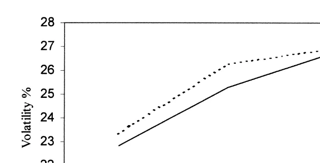
returns become more volatile.12Fig. 2 evidences that term structure of implied volatilities for call and put options is upward sloping. Empirical evidence indicates that upward sloping term structure is a characteristic of markets with lower
Ž . Ž .
volatility as in the United States , while high volatility markets notably Japan usually present downward-sloping term structures.13
4.3. Methodology
Ž
First of all, we identify the presence of eventual mispricings taking the value .
of Black and Scholes as the theoretical price using the historical and implied volatilities estimated in ty1 as a forecast of volatility at time t. Once an option appears to be undervalued–overvalued by the market, aAdelta hedgingBstrategy is simulated in an attempt to exploit the mispricing. TheAdeltaB is recalculated on a
Ž .
daily basis up to maturity excluding Bank Holidays and weekends . The hedging Ž . strategy takes place when the absolute value of the percentage deviation d of the
Ž . Ž .
actual price of the option OP from the theoretical price OTP is more than 15%, < <
in other words, when d)0.15. Each hedge is carried out on 10 contracts. It is assumed that the strategy to profit from the mispricing detected at time t takes
12 Ž .
Christie 1982 explains that when prices are low companies become more leveraged increasing both the required return and its variance.
13
Fig. 2. Term structure of volatility. The Figure evidences the variation of implied volatility as a function of option maturity for at-the-money options.
Ž .
place exactly at time t and at the same prices this is an Aex-postB test . The positions thus built up are maintained until maturity of the options. If it appears profitable within maturity to open more than one position, the equal sign positions are accumulated and opposite sign ones counterbalance one another to get the net position. The MIB30 index positions are then closed at maturity, at the settlement price of the contract, fixed, on the basis of a CONSOB deliberations, as equal to the value of the index calculated on the opening prices of its securities.14 It is assumed that the purchase of the option or of the index is financed by borrowing at the risk-free rate, and therefore involves the payment of interest. As evidenced in the previous analysis, the short sale of the option or of the index involves a cost deriving from the difference between the market interest rate and the repo rate at which the sale proceeds can be invested. We used as a proxy of this interest rate the bid rate. Apart from the cost due to payment of interest, the commission costs on the index and the options must also be considered. We recall from Section 3 that commission varies according to whether a trader of a certain importance or an individual investor is involved. It is assumed that, if the simulated strategies were actually implemented by professional arbitrageurs, the tariffs would be 10 000 ITL for option contracts and 5 index points for basket trading.
14
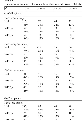
Table 3
Number of mispricings at various thresholds using different volatility estimates
< <d )5% )10% )15% )20% )25% )30%
Ž .a Call options
Call at the money
Hsd 113 70 44 23 14 5
61% 38% 24% 13% 8% 3%
WISDc 52 10 3 2 2 2
28% 5% 2% 1% 1% 1%
WISDpc 62 13 3 2 1 1
34% 7% 2% 1% 1% 1%
Call out of the money
Hsd 137 111 83 60 47 37
74% 60% 45% 33% 26% 20%
WISDc 80 34 16 8 5 4
43% 18% 9% 4% 3% 2%
WISDpc 104 54 31 20 9 6
57% 29% 17% 11% 5% 3%
Call in the money
Hsd 81 36 16 13 10 7
44% 20% 9% 7% 5% 4%
WISDc 40 20 16 13 10 8
22% 11% 9% 7% 5% 4%
WISDpc 46 20 15 14 8 7
25% 11% 8% 8% 4% 4%
Ž .b Put options
Put at the money
Hsd 133 87 63 48 37 28
72% 47% 34% 26% 20% 15%
WISDp 76 27 12 10 4 3
41% 15% 7% 5% 2% 2%
WISDpc 63 19 9 6 6 3
34% 10% 5% 3% 3% 2%
Put out of the money
Hsd 147 133 116 97 83 72
80% 72% 63% 53% 45% 39%
WISDp 89 53 31 17 12 10
48% 29% 17% 9% 7% 5%
WISDpc 107 54 40 29 20 13
58% 29% 22% 16% 11% 7%
Put in the money
Hsd 94 44 25 16 4 2
51% 24% 14% 9% 2% 1%
WISDp 53 16 8 5 2 2
Ž .
Table 3 continued
< <d )5% )10% )15% )20% )25% )30%
Ž .b Put options
WISDpc 43 12 9 4 2 2
23% 7% 5% 2% 1% 1%
The Table reports the number of mispricings both in absolute value and as a percentage of the total number of observations. Hsd is the Historical standard deviation; WISDc, WISDp are, respectively, the
Ž .
weighted implied volatilities calculated using three call option prices at different strike prices and three put option prices. WISDpc is the weighted implied volatilit y obtained using the three call price and the three put prices.
Running a trading simulation as described, we tested the MIBO30 market efficiency, verifying the possibility of achieve profits reducing the effects of the MIB30 index variations on the results of the strategy. The simulation undertaken permitted to overcome some of the already mentioned limitations inherent to the
Ž .
Black and Scholes model. In particular: i the Black and Scholes model was used in the strategy exclusively to identify overpriced and underpriced call options. Moreover, the threshold level for the difference between calculated and effective
Ž .
prices was purposely fixed at a high level 15% in order to account for Ž .
differences attributable to any inefficiency of the model. ii The dynamic hedging allows to account for eventual variations in the volatility of the index returns
Ž .
during the period and for the effective distribution of these returns; iii during the course of the trial, the transaction costs of both call trading and dealings in MIB30 indices were taken into account.15 The simulation also permitted to have some indication of the forecasting capacity of the two forecasts of the volatility utilised.
Ž< < Table 3a and b give the number of mispricings at various thresholds ds <ŽOTPyOP.rOP<)5%, 10%, 15%, 20%, 25%, 30% . It can be noted that, for. both call and put options, the highest number of arbitrage opportunities is discovered for options out of the money and the lowest number for options in the money. Moreover, the number of cases in which the mispricing exceeds 15% is quite restricted.
4.4. Empirical eÕidence
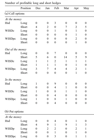
The simulation of the arbitrage strategies are based on estimates of historical and weighted implied volatilities. Table 4a and b gives the number of options, respectively, call and put, on which hedging was applied. The strategy consists in assuming a longrshort position in the option if it results to be undervalued or overvalued by the market.
15 Ž .
Table 4
Number of profitable long and short hedges
Position Dec Jan Feb Mar Apr May June July Aug Sept
Ž .a Call options
At the money
Hsd Long 0 0 3 0 0 0 0 0 0 2
Short 4 2 0 7 2 5 14 4 0 1
WISDc Long 0 0 1 0 1 0 0 0 0 0
Short 0 0 0 0 1 0 0 0 0 0
WISDpc Long 0 0 0 0 2 0 0 0 0 0
Short 0 0 0 0 1 0 0 0 0 0
Out of the money
Hsd Long 0 0 7 0 0 0 0 1 0 6
Short 5 6 0 14 5 9 19 6 3 2
WISDc Long 1 1 2 1 1 1 1 1 0 1
Short 1 1 1 0 1 0 1 0 1 0
WISDpc Long 3 7 4 4 2 1 4 3 0 0
Short 0 0 0 0 1 0 1 0 1 0
In the money
Hsd Long 1 0 9 0 0 0 0 0 1 0
Short 0 0 4 1 0 0 0 0 0 0
WISDc Long 1 0 8 1 1 0 0 0 1 0
Short 0 0 4 0 0 0 0 0 0 0
WISDpc Long 1 0 8 1 0 0 0 0 1 0
Short 0 0 4 0 0 0 0 0 0 0
Ž .b Put options
At the money
Hsd Long 0 0 4 0 1 0 0 0 0 2
Short 4 9 1 9 1 3 20 10 2 2
WISDp Long 0 2 2 0 2 1 0 1 0 1
Short 0 0 1 0 1 0 0 0 0 1
WISDpc Long 0 0 3 0 1 1 0 0 0 0
Short 0 0 1 0 0 0 2 0 0 1
Out of the money
Hsd Long 0 0 6 0 1 0 0 0 0 2
Short 7 13 1 17 12 14 22 19 7 5
WISDp Long 0 0 2 0 2 0 0 1 0 1
Short 3 3 5 1 4 0 4 2 2 1
WISDpc Long 0 0 3 0 2 0 0 0 0 0
Short 4 7 3 4 4 0 6 4 2 1
In the money
Hsd Long 0 0 1 1 1 0 0 0 0 0
Short 0 1 0 1 0 0 15 4 1 1
WISDp Long 0 2 1 1 2 0 0 0 0 0
Ž .
Table 4 continued
Position Dec Jan Feb Mar Apr May June July Aug Sept
Ž .b Put options
WISDpc Long 0 2 3 1 2 0 0 0 0 0
Short 0 0 1 0 0 0 0 0 0 0
Hsd is the Historical standard deviation; WISDc, WISDp are, respectively, the weighted implied
Ž .
volatilities calculated using three call option prices at different strike prices and three put option prices. WISDpc is the weighted implied volatility obtained using the three call price and the three put prices.
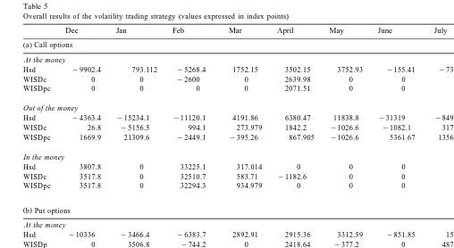
Overall results of the strategies are presented synthetically in Table 5a and b. Despite being quite controversial, these results do not indicate the possibility of realising systematic profits using a delta hedging strategy, whatever is the estimate used to forecast the effective volatility.16
Despite the strategy played on bothAin-the-moneyB call options and A out-of-the-moneyBput options always give positive results at the end of the whole period considered, monthly results present a high variability, with positive and negative signs. Moreover, results obtained for in the money call option, positive for almost all the sub-periods, have to be taken with caution. We can observe that the majority of the profits are concentrated in the month of February, when the index registered a strong and unexpected rise. This evidence indicates the sensibility of the portfolio to movements in the index. It should be kept in mind that the delta represents only a rough estimate of the price variation of the option as compared to the variation of the underlying security. For in the money options, the hedging error is particularly high. Therefore, these options are subjected to a wider distortion resulting from the movements of the MIB30 index. To this we must add that, although the risk of a lack of synchrony between the option price and the index price is minimised using a high-quality data set, this risk is higher when in the money options are involved. In fact, in the money options are the least liquid, with effective exchanges and related prices taking place intermittently. For these options, therefore, it is possible that the time lapse between the moment of disclosure of the index and that of the price of the option may be sufficient to determine an error in the calculation of the theoretical price. The risk of error in the case of in the money calls is such that it compensates for the profits obtainable by the arbitrage. In fact, even if in this case the error was favourable and led to profits, a different path of the index price movements could have led to different
Ž .
results. Taken as a whole, the two effects hedging error and lack of synchrony seem to diminish the results, without refuting the validity of the hypothesis of
16
()
Overall results of the volatility trading strategy values expressed in index points
Dec Jan Feb Mar April May June July Aug Sept Total
Ž .a Call options
At the money
Hsd y9902.4 793.112 y5268.4 1752.15 3502.15 3752.93 y155.41 y738.05 0 206.497 y6057.424
WISDc 0 0 y2600 0 2639.98 0 0 0 0 0 39.939
WISDpc 0 0 0 0 2071.51 0 0 0 0 0 2071.512
Out of the money
Hsd y4363.4 y15234.1 y11120.1 4191.86 6380.47 11838.8 y31319 y8499.5 y2350 3457.123 y47017.3 WISDc 26.8 y5156.5 994.1 273.979 1842.2 y1026.6 y1082.1 3174.47 28.883 y1336.00 y2260.8 WISDpc 1669.9 21309.6 y2449.1 y395.26 867.905 y1026.6 5361.67 13565.2 28.883 0 38932.3
In the money
Hsd 3807.8 0 33225.1 317.014 0 0 0 0 1549.2 0 38899.18 WISDc 3517.8 0 32510.7 583.71 y1182.6 0 0 0 1549.2 0 36978.96 WISDpc 3517.8 0 32294.3 934.979 0 0 0 0 1549.2 0 38296.35
Ž .b Put options
At the money
Hsd y10336 y3466.4 y6383.7 2892.91 2915.36 3312.59 y851.85 154.413 y85.54 1371.263 y10476.9 WISDp 0 3506.8 y744.2 0 2418.64 y377.2 0 4873.22 0 1271.612 10948.9 WISDpc 0 0 y2116.7 0 1451.35 y377.2 872.97 0 0 123.1449 y46.4
Out of the money
Hsd y13921.1 2980.5 y11048.3 11972.4 6687.14 7258.49 10672.7 557.405 y12.39 y3577.946 11568.8 WISDp y5230 5 y69.6 2095.5 2115.23 1056.89 0 892.891 2587.73 1086.2 y1161.17 3373.2 WISDpc y7783.2 1314.1 1126.3 7231.43 1266.72 0 1234.99 y545.61 1086.2 y909.502 4021.6
In the money
Hsd 0 y1970.28 y1883.4 1762.36 2645.53 0 y24172 y3914.8 y1346.5 y2824.17 y31703.3 WISDp 0 5496.8 5833.7 1415.59 4144.57 0 0 0 0 0 16890.8 WISDpc 0 4158.755 2626.893 1415.59 2746.42 0 0 0 0 0 10947.7
This table reports the results of the strategy obtained using different estimates of the index volatility. Hsd is the Historical standard deviation; WISDc, WISDp are, respectively, the weighted
Ž .
efficiency of the MIBO30 market. Results seem also to be consistent with the finding of many studies, asserting that the implied volatilities are better predictors
Ž
of future volatility than those obtained from historic price data Canina and .
Figlewski, 1993 . Despite that this finding needs further and more direct
investiga-Ž . Ž .
tion, we can observe that profits losses are generally higher lower when the volatility is predicted using the implied rather than the historical estimate.
5. Conclusions
The purpose of this study was to test the efficiency of the recently introduced Italian Index Option contract. The results obtained show that the market is on the whole efficient.
Ž .1 The put–call parity test, once the bid–ask spread and the transaction costs are taken into account, supports the hypothesis of market efficiency. In fact, the possibility of profitable hedges was encountered in only 2% of the cases with retail operators and, respectively, in 5% and 6% of the cases with institutional operators dealing in long or short hedges. Moreover, the presence of a very similar number of cases of profitable short and long hedges implicitly upholds the
Ž
hypothesis of efficiency of the market for securities lending at least for the 30 .
securities which constitute the MIB30 index . Alternatively, it may support the hypothesis that the market makers and dealers in securities do not make the hedge through the short-sale of the portfolio that replicates the index, but use predomi-nantly the future contract on the MIB30 index as a substitute.
Acknowledgements
The authors thank participants to theA11th Annual European Futures Research
Ž .
SymposiumB organised by the CBOT for useful insights. We also gratefully acknowledge the comments and suggestions of M. Bagella, E. Barone, Don M. Chance, A. Cybo Ottone, N. Di Noia, L. Mastroeni, W. Perraudin, D. Sabatini, C. Wolff and an anonymous referee. The usual disclaimer applies. The opinions expressed in this work do not necessarily reflect those of the Citibank and of the Prime Minister’s Office. We also thank the CONSOB for the data. Although this work was the result of the authors’ joint effort, Sections 1, 2.2, 3, 4.2 and 4.4 were written by Laura Cavallo and Sections 2.1, 4.1, 4.3 and 5 by Paolo Mammola. All tests were programmed in gauss by Laura Cavallo and are available upon request.
References
Barone, E., Cuoco, D., 1989. Il mercato dei contratti a premio in Italia, Rendiconti del Comitato per gli studi e la programmazione economica vol. XXVII, Alceo.
Barone, E.and Cuoco, D.,1991. Implied volatilities and arbitrage opportunities in the Italian options market, Working Paper.
Black, F., Scholes, M., 1971. The pricing of options and corporate liabilities. Journal of Political Economy 81, 637–659.
Black, F., Scholes, M., 1972. The valuation of Option Contracts and a test of market efficiency. Journal
Ž .
of Finance 27 2 , 399–417.
Cavallo, L.,1998. Option Market Efficiency and Pricing Models. Theoretical framework and empirical tests, PhD dissertation, University ofATor VergataB, Rome.
Cavallo, L.,1999. Optimal option replication with transaction costs: an empirical evaluation of several rehedging strategies, CEIS Working papers, n. 106, Rome.
Canina, L., Figlewski, S., 1993. The information content of implied volatility. The Review of Financial
Ž .
Studies 6 3 , 659–681.
Cavallo, L., Mammola, P. and Sabatini, D., 1999. Opzioni sul MIB30: proprieta fondamentali,`
Ž
volatility trading ed efficienza del mercato, CONSOB Italian Securities and Exchange
commis-.
sion Finance working papers n. 34.
Chiras, D.P., Manaster, S., 1978. The information content of option prices and a test of market efficiency. Journal of Financial Economics 6, 213–234.
Christie, A.A., 1982. The stochastic behaviour of common stock variances: value, leverage and interest-rate effects. Journal of Financial Economics 10, 407–432.
Ž .
Evnine, J., Rudd, A., 1985. Index options: the early evidence. Journal of Finance XL 3 . Fama, E., 1965. The behavior of stock market prices. Journal of Business 38, 34–105.
Finucane, T.J., 1991. Put call parity and expected returns. Journal of Financial and Quantitative
Ž .
Analysis 26 4 , 445–457.
French, K.R., 1980. Stock returns and the week-end effect. Journal of Financial Economics 8, 55–69. French, K., Roll, E., 1986. Stock return variances: the arrival of information and the reaction of traders.
Journal of Financial Economics 17, 5–26.
Galai, D., 1977. Tests of market efficiency of the Chicago board options exchange. Journal of Business
Ž .
50 2 , 167–197.
Gemmil, G., 1996. Did option traders anticipate the crash? Evidence from volatility smiles in the U.K.
Ž .
with U.S. comparisons. The Journal of Futures Markets 16 8 , 881–897.
Gould, J.P., Galai, D., 1974. Transactions costs and the relationship between put and call prices. The Journal of Financial Economics 1, 105–129.
Harvey, C.R., Whaley, R.E., 1992. Market volatility prediction and the efficiency of the S&P 100 index option market. Journal of Financial Economics 31, 43–73.
Joo, T.H., Dickinson, J.P., 1993. A test of the efficiency of the European options exchange. Applied Financial Economics 3, 175–181.
Klemkosky, R.C., Resnick, B.G., 1979. Put–call parity and market efficiency. The Journal of Finance
Ž .
XXXIV 5 .
MacBeth, J.D., Merville, J., 1979. An empirical examination of the Black–Scholes call option pricing model. The Journal of Finance 34, 1173–1186.
Merton, R.C., 1973. Theory of rational option pricing. The Bell Journal of Economics and Management Science 4, 141–183.
Nisbet, M., 1992. Put–call parity theory and an empirical test of the efficiency of the London traded options market. Journal of Banking and Finance 16, 381–403.
Phillips, S.M., Smith, C.W. Jr., 1980. Trading costs for listed options: the implications for market
Ž .
efficiency. Journal of Financial Economics 8 2 , 179–201.
Stoll, H.R., 1969. The relationship between put and call option prices. The Journal of Finance XXIV
Ž .5 .
Xu, -X., Taylor, S.J., 1995. Conditional volatility and the informational efficiency of the PHLX
Ž .